6.2 Solution

To me the shape that resembles the droplet the most is sphere. Luckily, it also got well defined formulas for surface area and volume (see the link above), so this is what we will use in our solution.

struct Sphere
    radius::Flt
    Sphere(r::Flt) = r <= 0 ? error("radius must be > 0") : new(r)
end

# formula from Wikipedia
function getVolume(s::Sphere)::Flt
    return (4/3) * pi * s.radius^3
end

# formula from Wikipedia
function getSurfaceArea(s::Sphere)::Flt
    return 4 * pi * s.radius^2
end

Now, let’s define a big lipid droplet with a radius of, let’s say, 10 [μm].

referenceDroplet = Sphere(10.0)

In the next step we will split this big droplet into a few smaller ones of equal sizes. Splitting the volume is easy, we just divide it by the number of droplets. However, we need a way to determine the size (radius) of each small droplet. Let’s try to transform the formula for a sphere’s volume and see if we can get a radius from that.

\[ v = \frac{4}{3} * \pi * r^3 \qquad{(4)}\]

If a = b, then b = a, so we may swap sides.

\[ \frac{4}{3} * \pi * r^3 = v \qquad{(5)}\]

The multiplication is commutative (the order does not matter), i.e. 2 * 3 * 4 is the same as 4 * 3 * 2 or 2 * 4 * 3, therefore we can rearrange elements on the left side of Equation 5 to:

\[ r^3 * \frac{4}{3} * \pi = v \qquad{(6)}\]

Now, one by one we can move *\(\frac{4}{3}\) and *\(\pi\) to the right side of Equation 6. Of course, we change the mathematical operation to the opposite (division instead of multiplication) and get:

\[ r^3 = v / \frac{4}{3} / \pi \qquad{(7)}\]

All that’s left to do is to move exponentiation (\(x^3\)) to the right side of Equation 7 while changing it to the opposite mathematical operation (cube root, i.e. \(\sqrt[3]{x}\)).

\[ r = \sqrt[3]{v / \frac{4}{3} / \pi} \qquad{(8)}\]

Now, you might wanted to quickly verify the solution using Symbolic.symbolic_linear_solve we met in Section 3.2. Unfortunately, we cannot use r^3 (r to the 3rd power) as an argument (and solve for r), since then it wouldn’t be a linear equation (to be linear the maximum power must be equal to 1) required by _linear_solve. We could have used other, more complicated solver, but instead we will keep things simple and apply a little trick:

import Symbolics as Sym

# fraction - 4/3, p - π, r3 - r^3, v - volume
Sym.@variables fraction p r3 v
Sym.symbolic_linear_solve(fraction * p * r3 ~ v, r3)

v / (fraction*p)

So, instead of writing the formula as it is, we just named our variables fraction, p, r3 and v. Anyway, according to Sym.symbolic_linear_solve \(r^3 = v / (\frac{4}{3} * \pi)\), which is actually the same as Equation 7 above [since e.g. 18 / 2 / 3 == 18 / (2 * 3)]. Ergo, we may be fairly certain we correctly solved Equation 7 and therefore Equation 8.

Once, we confirmed the validity of the formula in Equation 8, all that’s left to do is to translate it into Julia code.

function getSphere(volume::Flt)::Sphere
    # cbrt - fn that calculates cube root of a number
    radius::Flt = cbrt(volume / (4/3) / pi)
    return Sphere(radius)
end

Note: If there were no function for \(\sqrt[3]{x}\) you could easily define it yourself with: getCbrt(x) = x^(1/3) (here I used a single expression function for brevity) since \(\sqrt[n]{x} = x^{1/n}\).

Once we got that figured out, we evaluate the total area of the droplets of different size.

nDroplets = [1, 4, 8, 12]
totalVolumes = repeat([getVolume(referenceDroplet)], length(nDroplets))
individualVolumes = totalVolumes ./ nDroplets
droplets = getSphere.(individualVolumes)
radii = map(s -> s.radius, droplets)
individualSurfaceAreas = getSurfaceArea.(droplets)
totalSurfaceAreas = individualSurfaceAreas .* nDroplets

This seemed like a breeze thanks to the dot operators. We begin by by defining the nDroplets, i.e. the number of droplets that we will consider. Next, we divide their totalVolumes by their numbers (nDroplets) to get a volume of an individual droplet (individualVolumes). Based on the individual volumes we create the droplets of the appropriate radius (getSphere.(individualVolumes)). We also extract the radii for future use (the draw function below). Now, we calculate individualSurfaceAreas of our small droplets (getSurfaceArea.(droplets)) and then their totalSurfaceAreas. And we were able to achieve all that in only 7 lines of code.

Anyway, now, we can either examine the vectors (totalSurfaceAreas, radii, nDroplets, individualVolumes) one by one, or do one better and present them on a graph with e.g. CairoMakie (I’m not going to explain the code below, for reference see my previous book or CairoMakie tutorial).

import CairoMakie as Cmk

fig = Cmk.Figure();
ax = Cmk.Axis(fig[1, 1],
              title="Lipid droplet size vs. summaric surface area",
              xlabel="number of lipid droplets",
              ylabel="total surface area [μm²]", xticks=0:13);
Cmk.scatter!(ax, nDroplets, totalSurfaceAreas, markersize=radii .* 5,
             color="gold1", strokecolor="black");
Cmk.xlims!(ax, -3, 16);
Cmk.ylims!(ax, 800, 3000);
Cmk.text!(ax, nDroplets, totalSurfaceAreas .- 150,
    text=map(r -> "single droplet radius = $(round(r, digits=2)) [μm]",
             radii),
    fontsize=12, align=(:center, :center)
);
Cmk.text!(ax, nDroplets, totalSurfaceAreas .- 250,
          text=map((v, n) ->
              "volume ($n droplet/s) = $(round(Int, v)) [μm³]",
                   totalVolumes, nDroplets),
    fontsize=12, align=(:center, :center)
);
fig

Behold.

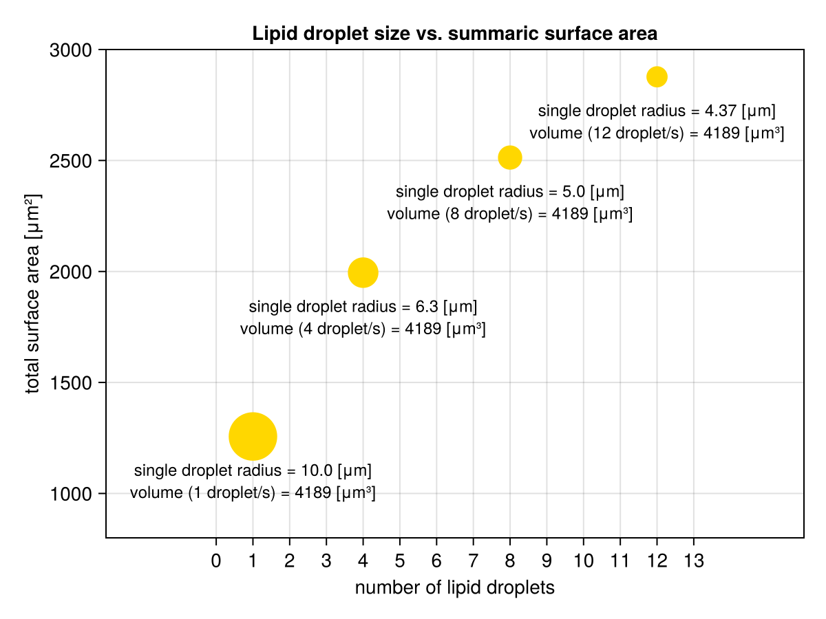
So it turns out that what they taught me in the school all those years ago is actually true. But only now I can finally see it. Nice.

Note: The above was an example of a geometrical property called surface-to-volume-ratio that applies to more than just the spheres and got its implications for many fields of science.