21.2 Solution

Let’s approach the problem step by step.

First let’s read the file’s contents (open and read were discussed in Section 17.2), uppercase all the characters (compare with Section 18.2) and preserve only letters from the English alphabet (filter).

# the file is roughly 31 KiB
# if necessary adjust the filePath
codedTxt = open("./code_snippets/shift/trarfvf.txt") do file
    read(file, Str)
end

codedTxt = uppercase(codedTxt)

function isUppercaseLetter(c::Char)::Bool
    return c in 'A':'Z'
end

codedTxt = filter(isUppercaseLetter, codedTxt)
first(codedTxt, 20)

VAGURORTVAAVATTBQPER

Time to get the letter counts and frequencies.

function getCounts(s::Str)::Dict{Char,Int}
    counts::Dict{Char, Int} = Dict()
    for char in s
        if haskey(counts, char)
            counts[char] = counts[char] + 1
        else
            counts[char] = 1
        end
    end
    return counts
end

function getFreqs(counts::Dict{Char, Int})::Dict{Char,Float64}
    total::Int = sum(values(counts))
    return Dict(k => v/total for (k, v) in counts)
end

function getFreqs(s::Str)::Dict{Char,Float64}
    return s |> getCounts |> getFreqs
end

The code is rather simple. Moreover it is quite similar to getCounts and getProbs that I discussed it in detail in my previous book so give it a sneak peak if you need a more thorough explanation (I apply DRY principle here).

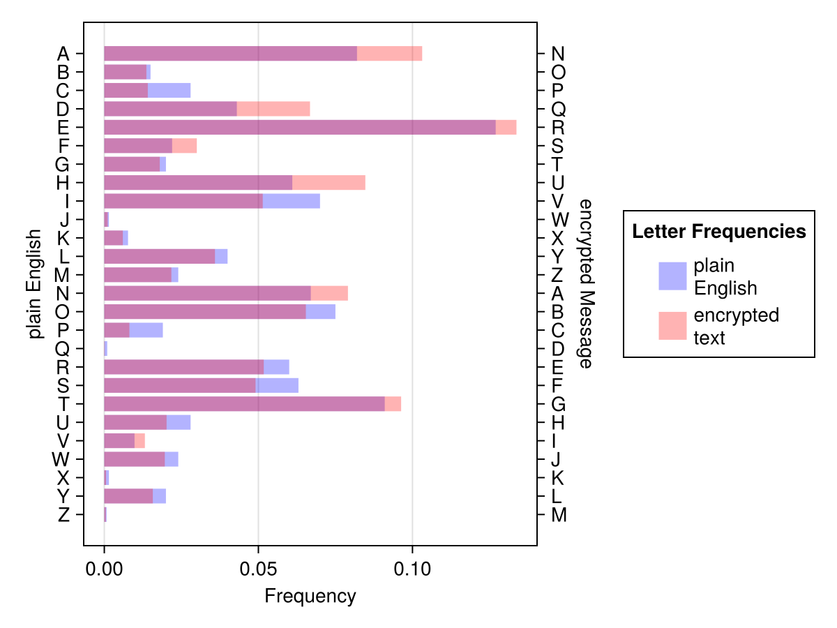
According to this Wikipedia’s page the letter that occurs most often in English is E (frequency: 0.127 or 12.7%, compare with this discussion). Time to see which letter is the most frequent in our encoded text.

codedLetFreqs = getFreqs(codedTxt)
[k => v for (k, v) in codedLetFreqs if v > 0.12]

'R' => 0.13374233128834356

And the winner is R. Interestingly, in the metal insides of a computer letters are represented as numbers (see, e.g. here). We can use this to our advantage and quickly obtain the shift.

'R' - 'E' # ASCII: 82 - 69

13

And so it turns out, that our encrypted message was coded with a shift cipher with the rotation of 13 (we will verify this finding in Section 22). If we were even more stubborn, we could display both the frequencies on a graph like Figure 12 (we do not expect the fit to be perfect).