32.2 Solution
Before we begin a few short definitions that we will use here (so that we are on the same page).
- principal - the money you borrow form a bank
- interest - the money you pay extra (except for the money you borrowed)
- interest rate - a percentage of principal which you will pay as interest
- installment - fixed monthly payment to the bank in order to cover you debt, part of it goes to pay off the principal and part to pay off the interest
Next, let’s use the formatting function from Section 31.2.
# getFormattedMoney from chapter: compound interest, modified
function fmt(money::Real, sep::Char=',',)::Str
    @assert money >= 0 "money must be >= 0"
    amount::Str = round(Int, money) |> string
    result::Str = ""
    counter::Int = 0
    for digit in reverse(amount) # digit is a single digit (type Char)
        if counter == 3
            result = sep * result
            counter = 0
        end
        result = digit * result
        counter += 1
    end
    return result * " USD"
end
Note: For another way to format a number to currency see Section 27.2.4.
Time to define a struct that will contain the data necessary to perform calculations for a given mortgage.
struct Mortgage
    principal::Real
    interestPercYr::Real
    numMonths::Int

    Mortgage(p::Real, i::Real, n::Int) = (
        p < 1 || i < 0 || n < 12 || n > 480) ?
        error("incorrect field values") : new(p, i, n)
end

mortgage1 = Mortgage(200_000, 6.49, 20*12)
mortgage2 = Mortgage(200_000, 4.99, 30*12)
Finally, we are ready to calculate our monthly payment to the bank.
# calculate c - money paid to the bank every month
function getInstallment(m::Mortgage)::Flt
    p::Real = m.principal
    r::Real = m.interestPercYr / 100 / 12
    n::Int = m.numMonths
    if r == 0
        return p / n
    else
        numerator::Flt = r * p * (1+r)^n
        denominator::Flt = ((1 + r)^n) - 1
        return numerator / denominator
    end
end
All the formulas are based on this Wikipedia page. Notice that the function’s arguments (Mortgage fields in getInstallment and the arguments to getPrincipalAfterMonth below) contain longer (more descriptive) names, whereas inside the functions we use the abbreviations (case insensitive) found in the above-mentioned formulas .
With that done, we can answer how much money we will have to pay to the bank every month for the duration of our mortgage.
(
    getInstallment(mortgage1) |> fmt,
    getInstallment(mortgage2) |> fmt
)
("1,490 USD", "1,072 USD")The money we still owe to the bank (principal) will change month after month (because every month we pay off a fraction of it with our installment), so let’s calculate that.
# amount of money owed after every month
function getPrincipalAfterMonth(prevPrincipal::Real,
                                interestPercYr::Real,
                                installment::Flt)::Flt
    @assert((prevPrincipal >= 0 && interestPercYr >= 0 && installment > 0),
            "incorrect argument values")
    p::Real = prevPrincipal
    r::Real = interestPercYr / 100 / 12
    c::Flt = installment
    return (1 + r) * p - c
end
Not much to explain here, just a simple rewrite of the formula into Julia’s code (first we increase the principal by interest, then we subtract the installment from it). Now we can estimate the principal owed to the bank each year.
# paying off mortgage year by year
# returns principal still owed every year
function getPrincipalOwedEachYr(m::Mortgage)::Vec{Flt}
    monthlyPayment::Flt = getInstallment(m)
    curPrincipal::Real = m.principal
    principalStillOwedYrs::Vec{Flt} = [curPrincipal]
    for month in 1:m.numMonths
        curPrincipal = getPrincipalAfterMonth(
            curPrincipal, m.interestPercYr, monthlyPayment)
        if month % 12 == 0
            push!(principalStillOwedYrs, curPrincipal)
        end
    end
    return principalStillOwedYrs
end
Here we calculate the principal owed after every month, and once a year (month % 12 == 0) we push it to a vector tracking its yearly change (principalStillOwedYrs). Let’s see how it works, if we did it right then in the end the principal should drop to zero (small rounding errors possible).
principals1 = getPrincipalOwedEachYr(mortgage1)
principals2 = getPrincipalOwedEachYr(mortgage2)
(
principals1[end],
principals2[end],
round(principals1[end], digits=2),
round(principals2[end], digits=2)
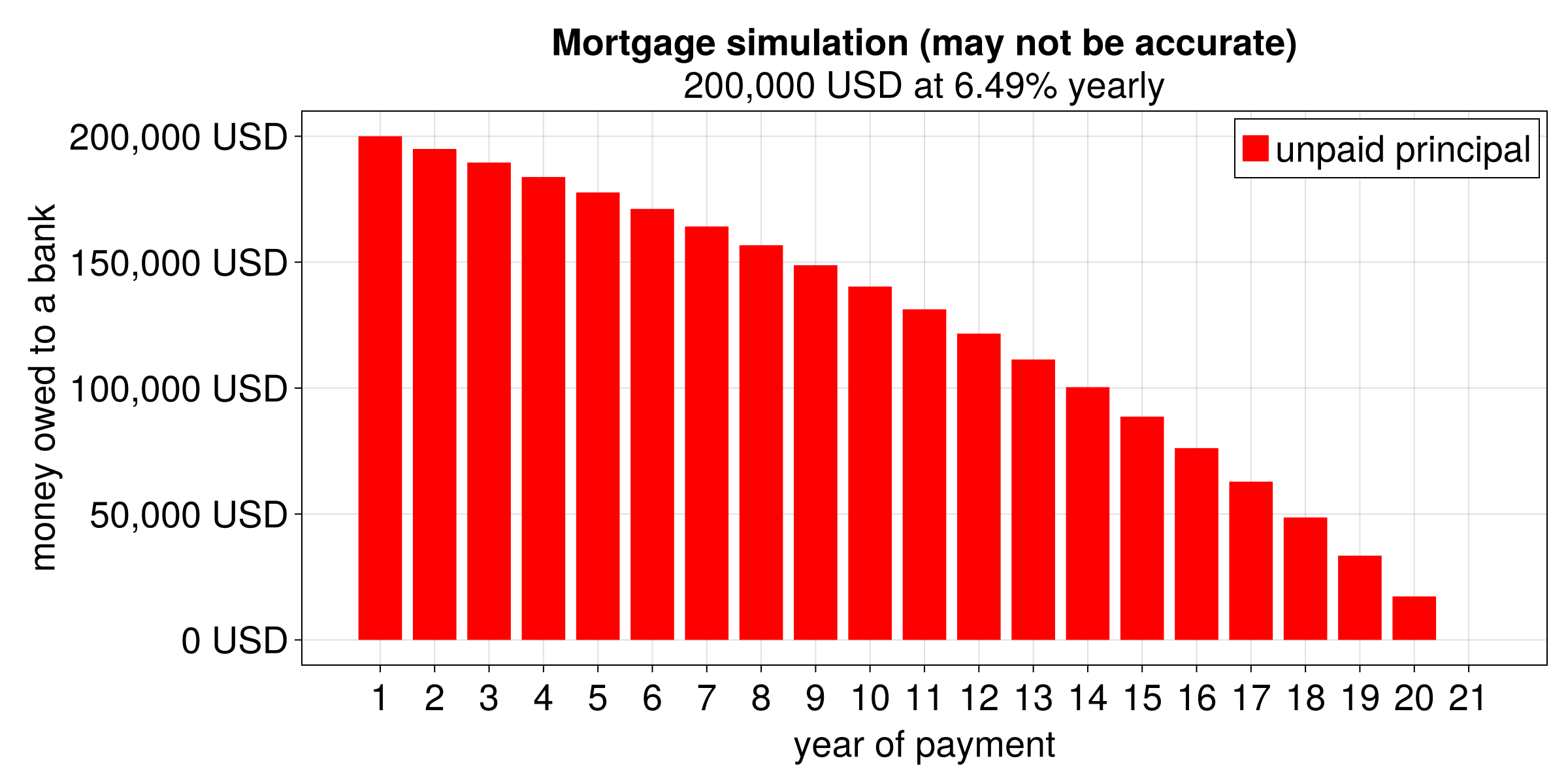
)(-1.1685642675729468e-8, -1.4030092643224634e-8, -0.0, -0.0)So how much principal we still owe to the bank at the beginning of year 15 in each scenario?
(
    principals1[15] |> fmt,
    principals2[15] |> fmt
)
("88,661 USD", "141,638 USD")Hmm, quite a lot (remember we borrowed $200,000 for 20 and 30 years). And when will this value drop \(\le\) 100,000 USD (\(\le\) half of what we borrowed)?
(
    findfirst(p -> p <= 100_000, principals1),
    findfirst(p -> p <= 100_000, principals2)
)
(15, 22)In general, for quite some time the money we pay to the bank mostly pay off the interest and not the principal, so that it drops slowly at first (see Figure 15).
To answer the last question (which mortgage is more worth it for us in terms of total payment and total interest) we’ll use a pie chart.
import CairoMakie as Cmk

function addPieChart!(m::Mortgage, fig::Cmk.Figure,
                      ax::Cmk.Axis, col::Int)::Nothing
    installment::Flt = getInstallment(m)
    totalInterest::Flt = installment * m.numMonths - m.principal
    yrs::Flt = round.(m.numMonths / 12, digits=2)
    colors::Vec{Str} = ["coral1", "turquoise2", "white", "white", "white"]
    lebels::Vec{Str} = ["interest = $(fmt(totalInterest))",
                        "principal = $(fmt(m.principal))",
                        "$(yrs) years, $(m.interestPercYr)% yearly",
                        "total cost = $(fmt(installment * m.numMonths))",
                        "monthly payment = $(fmt(installment))"]
    Cmk.pie!(ax, [totalInterest, m.principal], color=colors[1:2],
             radius=4, strokecolor=:white, strokewidth=5)
    Cmk.hidedecorations!(ax)
    Cmk.hidespines!(ax)
    Cmk.Legend(fig[3, col],
               [Cmk.PolyElement(color=c) for c in colors],
               lebels, valign=:bottom, halign=:center, fontsize=60,
               framevisible=false)
    return nothing
end
The function is rather simple. It adds a pie chart to an existing figure and axis. A point of notice, the colors used are ["coral1", "turquoise2", "white", "white", "white"]. The first two will be used to paint the circle. But all of them, will be used in the legend (Cmk.Legend). Hence, we used "white" for the values that are not in the circle (white color on a white background in the legend is basically invisible). We also used string interpolation where a simple interpolated value is placed after the dollar character ($) or in a more complicated case (a structure field, a calculation) it is put after the dollar character and within parenthesis (e.g. "$(2*3)").
Time to draw a comparison
function drawComparison(m1::Mortgage, m2::Mortgage)::Cmk.Figure
    fig::Cmk.Figure = Cmk.Figure(fontsize=18)
    ax1::Cmk.Axis = Cmk.Axis(
        fig[1:2, 1], title="Mortgage simulation\n(may not be accurate)",
        limits=(-5, 5, -5, 5), aspect=1)
    ax2::Cmk.Axis = Cmk.Axis(
        fig[1:2, 2], title="Mortgage simulation\n(may not be accurate)",
        limits=(-5, 5, -5, 5), aspect=1)
    Cmk.linkxaxes!(ax1, ax2)
    Cmk.linkyaxes!(ax1, ax2)
    addPieChart!(m1, fig, ax1, 1)
    addPieChart!(m2, fig, ax2, 2)
    return fig
end

drawComparison(mortgage1, mortgage2)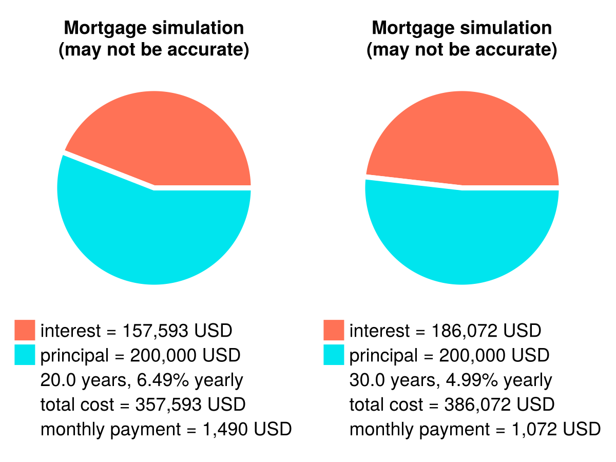
So it turns out that despite the higher interest rate of 6.49% overall we will pay less money to the bank for mortgage1. Therefore, if we are OK with the greater monthly payment (installment) then we may choose that one.
Of course, all the above was just a programming exercise, not a financial advice. Moreover, the simulation is likely to be inaccurate (to a various extent) for many reasons. For instance, a bank may calculate the interest every day, and not every month, in that case you will pay more. Compare with the simple example below and the compound interest from Section 31.2.1.
# 6% yearly, after 1 year
(
    200_000 * (1 + 0.06) |> fmt, # capitalized yearly
    200_000 * (1 + (0.06/12))^12 |> fmt, # capitalized monthly
    200_000 * (1 + (0.06/365))^365 |> fmt, # capitalized daily
)
("212,000 USD", "212,336 USD", "212,366 USD")Anyway, once you know what’s going on, it should be easier to modify the program to reflect a particular scenario more closely.