7.5 Correlation Pitfalls
The Pearson correlation coefficient is pretty useful (especially in connection with the Student’s t-test), but it shouldn’t be applied thoughtlessly.
Let’s take a look at the Anscombe’s quartet.
import RDatasets as RD

anscombe = RD.dataset("datasets", "anscombe")
first(anscombe, 5)
| X1 | X2 | X3 | X4 | Y1 | Y2 | Y3 | Y4 |
|---|---|---|---|---|---|---|---|
| 10.0 | 10.0 | 10.0 | 8.0 | 8.04 | 9.14 | 7.46 | 6.58 |
| 8.0 | 8.0 | 8.0 | 8.0 | 6.95 | 8.14 | 6.77 | 5.76 |
| 13.0 | 13.0 | 13.0 | 8.0 | 7.58 | 8.74 | 12.74 | 7.71 |
| 9.0 | 9.0 | 9.0 | 8.0 | 8.81 | 8.77 | 7.11 | 8.84 |
| 11.0 | 11.0 | 11.0 | 8.0 | 8.33 | 9.26 | 7.81 | 8.47 |
The data frame is a part of RDatasets that contains a collection of standard data sets used with the R programming language. The data frame was carefully designed to demonstrate the perils of relying blindly on correlation coefficients.
fig = Cmk.Figure()
i = 0
for r in 1:2 # r - row
    for c in 1:2 # c - column
        i += 1
        xname = string("X", i)
        yname = string("Y", i)
        xs = anscombe[:, xname]
        ys = anscombe[:, yname]
        cor, pval = getCorAndPval(xs, ys)
        ax = Cmk.Axis(fig[r, c],
                      title=string("Figure ", "ABCD"[i]),
                      xlabel=xname, ylabel=yname,
                      limits=(0, 20, 0, 15))
        Cmk.scatter!(ax, xs, ys)
        Cmk.text!(ax, 9, 3, text="cor(x, y) = $(round(cor, digits=2))")
        Cmk.text!(ax, 9, 1, text="p-val = $(round(pval, digits=4))")
    end
end

fig
There’s not much to explain here. The only new part is string function that converts its elements to strings (if they aren’t already) and glues them together into a one long string. The rest is just plain drawing with CairoMakie. Still, take a look at the picture below
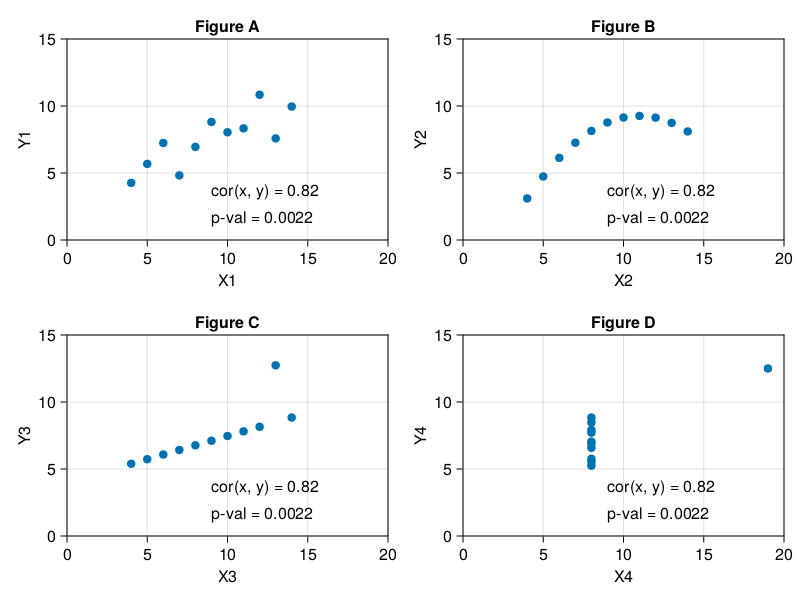
All the sub-figures from Figure 29 depict different relation types between the X and Y variables, yet the correlations and p-values are the same. Two points of notice here. In Figure B the points lie in a perfect order on a curve. So, in a perfect word the correlation coefficient should be equal to 1. Yet it is not, as it only measures the spread of the points around an imaginary straight line. Moreover, correlation is sensitive to outliers. In Figure D the X and Y variables appear not to be associated at all (for X = 8, Y can take any value). Again, in the perfect world the correlation coefficient should be equal to 0. Still, the outlier on the far right (that in real life may have occurred by a typographical error) pumps it up to 0.82 (or what we could call a very strong correlation). Lesson to be learned here, don’t trust the numbers, and whenever you can draw a scatter plot to double check them. And remember, “All models are wrong, but some are useful”.
Other pitfalls are also possible. For instance, imagine you measured body and tail length of a certain species of mouse, here are your results.
# if you are in 'code_snippets' folder, then use: "./ch07/miceLengths.csv"
# if you are in 'ch07' folder, then use: "./miceLengths.csv"
miceLengths = Csv.read(
    "./code_snippets/ch07/miceLengths.csv",
    Dfs.DataFrame)
first(miceLengths, 5)
| bodyCm | tailCm | sex |
|---|---|---|
| 11.3 | 2.55 | f |
| 11.18 | 2.22 | f |
| 9.42 | 2.54 | f |
| 9.21 | 2.2 | f |
| 9.97 | 2.63 | f |
You are interested to know if the tail length is associated with the body length of the animals.
getCorAndPval(miceLengths.bodyCm, miceLengths.tailCm)(0.8899347709623199, 1.5005298337200657e-7)Clearly it is and even very strongly. Or is it? Well, let’s take a look
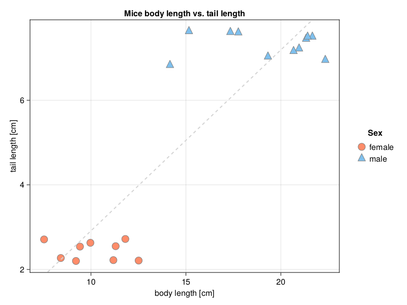
It turns out that we have two clusters of points. In both of them the points seem to be randomly scattered. This could be confirmed by testing correlation coefficients for the clusters separately.
isFemale(value) = value == "f"
isMale(value) = value == "m"

# fml - female mice lengths
# mml - male mice lengths
fml = miceLengths[isFemale.(miceLengths.sex), :] # choose only females
mml = miceLengths[isMale.(miceLengths.sex), :] # choose only males

(
    getCorAndPval(fml.bodyCm, fml.tailCm),
    getCorAndPval(mml.bodyCm, mml.tailCm)
)
((-0.1593819718041706, 0.6821046994037891),
(-0.02632446813765734, 0.9387606491398499))Note: The above code snippet uses a single expression functions in the form
functionName(argument) = returnedValueandBoolean indexing (isFemale.(miceLengths.sex)andisMale.(miceLengths.sex)) that was discussed briefly in Section 3.3.6 and Section 3.3.7.
Alternatively, you could read the documentation for the functionality built into DataFrames.jl to obtain the desired insight. Doing so takes time, effort, and causes irritation at first (trust me, I know). Still, there are no shortcuts to any place worth going. So, you may decide to use Dfs.groupby and Dfs.combine to get a similar result.
# gDf - grouped data frame
Dfs.groupby(miceLengths, :sex) |>
    gDf -> Dfs.combine(gDf, [:tailCm, :bodyCm] => Stats.cor => :r)
| sex | r |
|---|---|
| f | -0.1593819718041706 |
| m | -0.02632446813765729 |
Note: You could replace
Stats.corwithgetCorAndPvalin the snippet above. This should work if you changed the signature of the function fromgetCorAndPval(v1::Vector{<:Real}, v2::Vector{<:Real})togetCorAndPval(v1::AbstractVector{<:Real}, v2::Abstractvector{<:Real})first. A more comprehensiveDataFramestutorial can be found, e.g. here (if you don’t know what to do with*.ipynbfiles then you may just click on any of them to see its content in a web browser).
Anyway, the Pearson correlation coefficients are small and not statistically significant (p > 0.05). But since the two clusters of points lie on the opposite corners of the graph, then the overall correlation measures their spread alongside the imaginary dashed line in Figure 30. This inflates the value of the coefficient (compare with the explanation for z1, z2 and jitter in Section 7.4). Therefore, it is always good to inspect a graph (scatter plot) to see if there are any clusters of points. The clusters are usually a result of some grouping present in the data (either different experimental groups/treatments or due to some natural grouping). Sometimes we may be unaware of the groups in our data set. Still, if we do know about them, then it is a good idea to inspect the overall correlation and the correlation coefficient for each of the groups separately.
As the last example let’s take a look at this data frame.
# if you are in 'code_snippets' folder, then use: "./ch07/candyBars.csv"
# if you are in 'ch07' folder, then use: "./candyBars.csv"
candyBars = Csv.read(
    "./code_snippets/ch07/candyBars.csv",
    Dfs.DataFrame)
first(candyBars, 5)
| total | carb | fat |
|---|---|---|
| 44.49 | 30.23 | 9.67 |
| 48.39 | 29.31 | 12.48 |
| 49.83 | 30.95 | 10.58 |
| 40.51 | 25.22 | 9.89 |
| 44.51 | 29.45 | 10.15 |
Here, we got a data set on composition of different chocolate bars. You are interested to see if the carbohydrate (carb) content in bars is associated with their fat mass.
getCorAndPval(candyBars.carb, candyBars.fat)(0.12176486958519653, 0.7375535843598793)And it appears it is not. OK, no big deal, and what about carb and total mass of a candy bar?
getCorAndPval(candyBars.carb, candyBars.total)(0.822779226943004, 0.0034638410860259317)Now we got it. It’s big (r > 0.8) and it’s real (\(p \le 0.05\)). But did it really make sense to test that?
If we got a random variable aa then it is going to be perfectly correlated with itself.
Rand.seed!(321)
aa = Rand.rand(Dsts.Normal(100, 15), 10)

getCorAndPval(aa, aa)
(1.0, 0.0)On the other hand it shouldn’t be correlated with another random variable bb.
bb = Rand.rand(Dsts.Normal(100, 15), 10)

getCorAndPval(aa, bb)
(0.19399997195558746, 0.5912393958185727)Now, if we add the two variables together we will get the total (cc), that will be correlated with both aa and bb.
cc = aa .+ bb

(
    getCorAndPval(aa, cc),
    getCorAndPval(bb, cc)
)
((0.7813386818990972, 0.007608814877251513),
(0.763829856046036, 0.010120085355359132))This is because while correlating aa with cc we are partially correlating aa with itself (aa .+ bb). In general, the greater portion of cc our aa makes the greater the correlation coefficient. So, although possible, it makes little logical sense to compare a part of something with its total. Therefore, in reality running getCorAndPval(candyBars.carb, candyBars.total) makes no point despite the interesting result it seems to produce.