5.4 One-way ANOVA

One-way ANOVA is a technique to compare two or more groups of continuous data. It allows us to tell if all the groups are alike or not based on the spread of the data around the mean(s).

Let’s start with something familiar. Do you still remember our tennis players Peter and John from Section 4.7.1. Well, guess what, they work at two different biological institutes. The institutes independently test a new weight reducing drug, called drug Y, that is believed to reduce body weight of an animal by roughly 23%. The drug administration is fairly simple. You just dilute it in water and leave it in a cage for mice to drink it.

So both our friends independently run the following experiment: a researcher takes eight mice, writes at random numbers at their tails (1:8), and decides that the mice 1:4 will drink pure water, and the mice 5:8 will drink water with the drug. After a week body weights of all mice are recorded.

As said, Peter and John run the experiments independently not knowing one about the other. After a week Peter noticed that he messed things up and did not give the drug to mice (when diluted the drug is colorless and by accident he took the wrong bottle). It happened, still let’s compare the results that were obtained by both our friends.

import Random as Rand

# Peter's mice, experiment 1 (ex1)
Rand.seed!(321)
ex1BwtsWater = Rand.rand(Dsts.Normal(25, 3), 4)
ex1BwtsPlacebo = Rand.rand(Dsts.Normal(25, 3), 4)

# John's mice, experiment 2 (ex2)
ex2BwtsWater = Rand.rand(Dsts.Normal(25, 3), 4)
ex2BwtsDrugY = Rand.rand(Dsts.Normal(25 * 0.77, 3), 4)

In Peter’s case both mice groups came from the same population Dsts.Normal(25, 3) (\(\mu = 25\), \(\sigma = 3\)) since they both ate and drunk the same stuff. For need of different name the other group is named placebo.

In John’s case the other group comes from a different distribution (e.g. the one where body weight is reduced on average by 23%, hence \(\mu = 25 * 0.77\)).

Let’s see the results side by side on a graph.

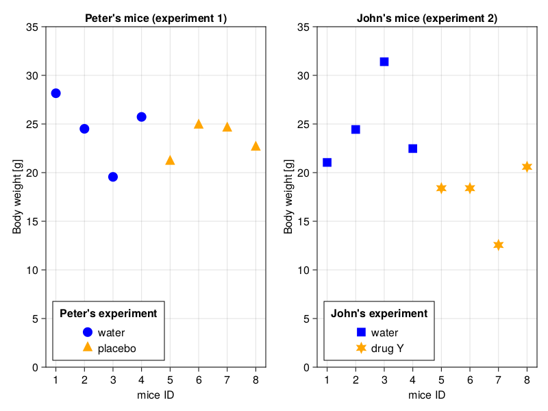
I don’t know about you, but my first impression is that the data points are more scattered around in John’s experiment. Let’s add some means to the graph to make it more obvious.

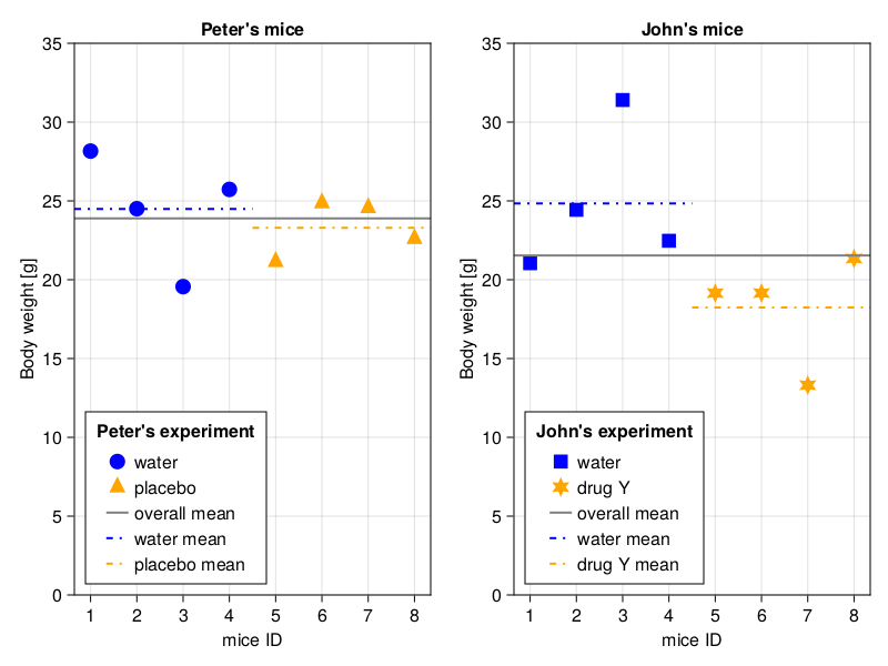
Indeed, with the lines (especially the overall means) the difference in spread of the data points seems to be even more evident. Notice an interesting fact, in the case of water and placebo the group means are closer to each other, and to the overall mean. This makes sense, after all the animals ate and drunk exactly the same stuff, so they belong to the same population. On the other hand in the case of the two populations (water and drugY) the group means differ from the overall mean (again, think of it for a moment and convince yourself that it makes sense). Since we got Julia on our side we could even try to express this spread of data with numbers. First, the spread of data points around the group means

function getAbsDiffs(v::Vector{<:Real})::Vector{<:Real}
    return abs.(Stats.mean(v) .- v)
end

function getAbsPointDiffsFromGroupMeans(
    v1::Vector{<:Real}, v2::Vector{<:Real})::Vector{<:Real}
    return vcat(getAbsDiffs(v1), getAbsDiffs(v2))
end

ex1withinGroupsSpread = getAbsPointDiffsFromGroupMeans(
    ex1BwtsWater, ex1BwtsPlacebo)
ex2withinGroupsSpread = getAbsPointDiffsFromGroupMeans(
    ex2BwtsWater, ex2BwtsDrugY)

ex1AvgWithinGroupsSpread = Stats.mean(ex1withinGroupsSpread)
ex2AvgWithingGroupsSpread = Stats.mean(ex2withinGroupsSpread)

(ex1AvgWithinGroupsSpread, ex2AvgWithingGroupsSpread)

(1.941755009754579, 2.87288915817597)

The code is pretty simple. Here we calculate the distance of data points around the group means. Since we are not interested in a sign of a difference [+ (above), - (below) the mean] we use abs function. We used a similar methodology when we calculated absDiffsStudA and absDiffsStudB in Section 4.6. This is as if we measured the distances from the group means in Figure 16 with a ruler and took the average of them. The only new part is the vcat function. All it does is it glues two vectors together, like: vcat([1, 2], [3, 4]) gives us [1, 2, 3, 4]. Anyway, the average distance of a point from a group mean is 1.9 [g] for experiment 1 (left panel in Figure 16). For experiment 2 (right panel in Figure 16) it is equal to 2.9 [g]. That is nice, as it follows our expectations. However, AvgWithinGroupsSpread by itself is not enough since sooner or later in experiment 1 (hence prefix ex1-) we may encounter (a) population(s) with a wide natural spread of the data. Therefore, we need a more robust metric.

This is were the average spread of group means around the overall mean could be useful. Let’s get to it, we will start with these functions

function repVectElts(v::Vector{T}, times::Vector{Int})::Vector{T} where T
    @assert (length(v) == length(times)) "length(v) not equal length(times)"
    @assert all(map(x -> x > 0, times)) "times elts must be positive"
    result::Vector{T} = Vector{eltype(v)}(undef, sum(times))
    currInd::Int = 1
    for i in eachindex(v)
        for _ in 1:times[i]
            result[currInd] = v[i]
            currInd += 1
        end
    end
    return result
end

function getAbsGroupDiffsFromOverallMean(
    v1::Vector{<:Real}, v2::Vector{<:Real})::Vector{<:Real}
    overallMean::Float64 = Stats.mean(vcat(v1, v2))
    groupMeans::Vector{Float64} = [Stats.mean(v1), Stats.mean(v2)]
    absGroupDiffs::Vector{<:Real} = abs.(overallMean .- groupMeans)
    absGroupDiffs = repVectElts(absGroupDiffs, map(length, [v1, v2]))
    return absGroupDiffs
end

The function repVectElts is a helper function. It is slightly complicated and I will not explain it in detail. Just treat it as any other function from a library. A function you know only by name, input, and output. A function that you are not aware of its insides (of course if you really want you can figure them out by yourself). All it does is it takes two vectors v and times, then it replicates each element of v a number of times specified in times like so: repVectElts([10, 20], [1, 2]) output [10, 20, 20]. And this is actually all you care about right now.

As for the getAbsGroupDiffsFromOverallMean it does exactly what it says. It subtracts group means from the overall mean (overallMean .- groupMeans) and takes absolute values of that [abs.(]. Then it repeats each difference as many times as there are observations in the group repVectElts(absGroupDiffs, map(length, [v1, v2])) (as if every single point in a group was that far away from the overall mean). This is what it returns to us.

OK, time to use the last function, behold

ex1groupSpreadFromOverallMean = getAbsGroupDiffsFromOverallMean(
    ex1BwtsWater, ex1BwtsPlacebo)
ex2groupSpreadFromOverallMean = getAbsGroupDiffsFromOverallMean(
    ex2BwtsWater, ex2BwtsDrugY)

ex1AvgGroupSpreadFromOverallMean = Stats.mean(ex1groupSpreadFromOverallMean)
ex2AvgGroupSpreadFromOverallMean = Stats.mean(ex2groupSpreadFromOverallMean)

(ex1AvgGroupSpreadFromOverallMean, ex2AvgGroupSpreadFromOverallMean)

(0.597596847858199, 3.6750594521844278)

OK, we got it. The average group mean spread around the overall mean is 0.6 [g] for experiment 1 (left panel in Figure 16) and 3.7 [g] for experiment 2 (right panel in Figure 16). Again, the values are as we expected them to be based on our intuition.

Now, we can use the obtained before AvgWithinGroupSpread as a reference point for AvgGroupSpreadFromOverallMean like so

LStatisticEx1 = ex1AvgGroupSpreadFromOverallMean / ex1AvgWithinGroupsSpread
LStatisticEx2 = ex2AvgGroupSpreadFromOverallMean / ex2AvgWithingGroupsSpread

(LStatisticEx1, LStatisticEx2)

(0.3077611979143188, 1.2792207599536367)

Here, we calculated a so called L-Statistic (LStatistic). I made the name up, because that is the first name that came to my mind. Perhaps it is because my family name is Lukaszuk or maybe because I’m selfish. Anyway, the higher the L-statistic (so the ratio of group spread around the overall mean to within group spread) the smaller the probability that such a big difference was caused by a chance alone (hmm, I think I said something along those lines in one of the previous chapters). If only we could reliably determine the cutoff point for my LStatistic.

Luckily, there is no point for us to do that since one-way ANOVA relies on a similar metric called F-statistic (BTW. Did I mention that the ANOVA was developed by Ronald Fisher? Of course, in that case others bestowed the name in his honor). Observe. First, experiment 1:

Htests.OneWayANOVATest(ex1BwtsWater, ex1BwtsPlacebo)

One-way analysis of variance (ANOVA) test
-----------------------------------------
Population details:
    parameter of interest:   Means
    value under h_0:         "all equal"
    point estimate:          NaN

Test summary:
    outcome with 95% confidence: fail to reject h_0
    p-value:                     0.5738

Details:
    number of observations: [4, 4]
    F statistic:            0.353601
    degrees of freedom:     (1, 6)

Here, my made up LStatistic was 0.31 whereas the F-Statistic is 0.35, so kind of close. Chances are they measure the same thing but using slightly different methodology. Here, the p-value (p > 0.05) demonstrates that the groups may come from the same population (or at least that we do not have enough evidence to claim otherwise).

OK, now time for experiment 2:

Htests.OneWayANOVATest(ex2BwtsWater, ex2BwtsDrugY)

One-way analysis of variance (ANOVA) test
-----------------------------------------
Population details:
    parameter of interest:   Means
    value under h_0:         "all equal"
    point estimate:          NaN

Test summary:
    outcome with 95% confidence: reject h_0
    p-value:                     0.0428

Details:
    number of observations: [4, 4]
    F statistic:            6.56001
    degrees of freedom:     (1, 6)

Here, the p-value (\(p \le 0.05\)) demonstrates that the groups come from different populations (the means of those populations differ). As a reminder, in this case my made up L-Statistic (LStatisticEx2) was 1.28 whereas the F-Statistic is 6.56, so this time it is more distant. The differences stem from different methodology. For instance, just like in Section 4.6 here (LStatisticEx2) we used abs function as our power horse. But do you remember, that statisticians love to get rid of the sign from a number by squaring it. Anyway, let’s rewrite our functions in a more statistical manner.

# compare with our getAbsDiffs
function getSquaredDiffs(v::Vector{<:Real})::Vector{<:Real}
    return (Stats.mean(v) .- v) .^ 2
end

# compare with our getAbsPointDiffsFromOverallMean
function getResidualSquaredDiffs(
    v1::Vector{<:Real}, v2::Vector{<:Real})::Vector{<:Real}
    return vcat(getSquaredDiffs(v1), getSquaredDiffs(v2))
end

# compare with our getAbsGroupDiffsAroundOverallMean
function getGroupSquaredDiffs(
    v1::Vector{<:Real}, v2::Vector{<:Real})::Vector{<:Real}
    overallMean::Float64 = Stats.mean(vcat(v1, v2))
    groupMeans::Vector{Float64} = [Stats.mean(v1), Stats.mean(v2)]
    groupSqDiffs::Vector{<:Real} = (overallMean .- groupMeans) .^ 2
    groupSqDiffs = repVectElts(groupSqDiffs, map(length, [v1, v2]))
    return groupSqDiffs
end

Note: In reality functions in statistical packages probably use a different formula for getGroupSquaredDiffs (they do not replicate groupSqDiffs). Still, I like my explanation better, so I will leave it as it is.

The functions are very similar to the ones we developed earlier. Of course, instead of abs.( we used .^2 to get rid of the sign. Here, I adopted the names (group sum of squares and residual sum of squares) that you may find in a statistical textbook/software.

Now we can finally calculate averages of those squares and the F-statistics itself with the following functions

function getResidualMeanSquare(
    v1::Vector{<:Real}, v2::Vector{<:Real})::Float64
    residualSquaredDiffs::Vector{<:Real} = getResidualSquaredDiffs(v1, v2)
    return sum(residualSquaredDiffs) / getDf(v1, v2)
end

function getGroupMeanSquare(
    v1::Vector{<:Real}, v2::Vector{<:Real})::Float64
    groupSquaredDiffs::Vector{<:Real} = getGroupSquaredDiffs(v1, v2)
    groupMeans::Vector{Float64} = [Stats.mean(v1), Stats.mean(v2)]
    return sum(groupSquaredDiffs) / getDf(groupMeans)
end

function getFStatistic(v1::Vector{<:Real}, v2::Vector{<:Real})::Float64
    return getGroupMeanSquare(v1, v2) / getResidualMeanSquare(v1, v2)
end

Again, here I tried to adopt the names (group mean square and residual mean square) that you may find in a statistical textbook/software. Anyway, notice that in order to calculate MeanSquares we divided our sum of squares by the degrees of freedom (we met this concept and developed the functions for its calculation in Section 5.2 and in Section 5.3.2). Using degrees of freedom (instead of length(vector) like in the arithmetic mean) is usually said to provide better estimates of the desired values when the sample size(s) is/are small.

OK, time to verify our functions for the F-statistic calculation.

(
    getFStatistic(ex1BwtsWater, ex1BwtsPlacebo),
    getFStatistic(ex2BwtsWater, ex2BwtsDrugY),
)

(0.3536010850042917, 6.560010563323356)

To me, they look similar to the ones produced by Htests.OneWayANOVATest before, but go ahead scroll up and check it yourself. Anyway, under \(H_{0}\) (all groups come from the same population) the F-statistic (so \(\frac{groupMeanSq}{residMeanSq}\)) got the F-Distribution (a probability distribution), hence we can calculate the probability of obtaining such a value (or greater) by chance and get our p-value (similarly as we did in Section 4.6.2 or in Section 5.2). Based on that we can deduce whether samples come from the same population (p > 0.05) or from different populations (\(p \le 0.05\)). Ergo, we get to know if any group (means) differ(s) from the other(s).