Statistics intro - Solutions - Romeo and Julia, where Romeo is Basic Statistics

4.9 Statistics intro - Solutions

In this sub-chapter you will find exemplary solutions to the exercises from the previous section.

4.9.1 Solution to Exercise 1

The easiest way to solve this problem is to reduce it to a simpler one.

If the PIN number were only 1-digit, then the total number of possibilities would be equal to 10 (numbers from 0 to 9).

For a 2-digit PIN the pattern would be as follow:

So, for every number in the first location there are 10 numbers (0-9) in the second location. Therefore in total we got numbers in the range 00-99, or to write it mathematically 10 * 10 different numbers (numbers per pos. 1 * numbers per pos. 2).

By extension the total number of possibilities for a 4-digit PIN is:

# (method1, method2, method3)
(10 * 10 * 10 * 10, 10^4, length(0:9999))

(10000, 10000, 10000)

So 10’000 numbers. Therefore the probability for a random number being the right one is 1/10_000 = 0.0001

Similar methodology is used to assess the strength of a password to an internet website.

4.9.2 Solution to Exercise 2

OK, so let’s reduce the problem before we solve it.

If I had only 1 beer and 1 label then there is only one way to do it. The label in my hand goes to the beer in front of me.

For 2 labels and 2 beer it goes like this:

a b
b a

I place one of two labels on a first beer, and I’m left with only 1 label for the second beer. So, 2 possibilities in total.

For 3 labels and 3 beer the possibilities are as follow:

a b c
a c b

b a c
b c a

c a b
c b a

So here, for the first beer I can assign any of the three labels (a, b, or c). Then I move to the second beer and have only two labels left in my hand (if the first got a, then the second can get only b or c). Then I move to the last beer with the last label in my hand (if the first two were a and b then I’m left with c). In total I got 3 * 2 * 1 = 6 possibilities.

It turns out this relationship holds also for bigger numbers. In mathematics it can be calculated using the factorial function that is already implemented in Julia (see the docs).

Still, for practice we’re gonna implement one on our own with the foreach we met in Section 3.6.4.

function myFactorial(n::Int)::Int
    @assert n > 0 "n must be positive"
    product::Int = 1
    foreach(x -> product *= x, 1:n)
    return product
end

myFactorial(6)

720

Note: You may also just use Julia’s prod function, e.g. prod(1:6) = 720. Still, be aware that factorial numbers grow pretty fast, so for bigger numbers, e.g. myFactorial(20) or above you might want to change the definition of myFactorial to use BigInt that we met in Section 3.9.5.

So, the probability that a person correctly labels 6 beer at random is round(1/factorial(6), digits=5) = 0.00139 = 1/720.

I guess that is the reason why out of 7 people that attempted to correctly label 6 beer the results were as follows:

one person correctly labeled 0 beer
five people correctly labeled 1 beer
one person correctly labeled 2 beer

I leave the conclusions to you.

4.9.3 Solution to Exercise 3

OK, for the original tennis example (see Section 4.7.1) we answered the question by using a computer simulation first (Section 4.7.2). For a change, this time we will start with a ‘purely mathematical’ calculations. Ready?

In order to get the result of 1-5 for Peter we would have to get a series of games like this one:

# 0 - John's victory, 1 - Peter's victory
0 1 1 1 1 1

Probability of either John or Peter winning under \(H_{0}\) (assumption that they play equally well) is \(\frac{1}{2}\) = 0.5. So here we got a conjunction of probabilities (John won AND Peter won AND Peter won AND …). According to what we’ve learned in Section 4.3.1 we should multiply the probabilities by each other.

Therefore, the probability of the result above is 0.5 * 0.5 * 0.5 * ... or 0.5 ^ 6 = 0.015625. But wait, there’s more. We can get such a result (1-5 for Peter) in a few different ways, i.e.

0 1 1 1 1 1
# or
1 0 1 1 1 1
# or
1 1 0 1 1 1
# or
1 1 1 0 1 1
# or
1 1 1 1 0 1
# or
1 1 1 1 1 0

Note: For a big number of games it is tedious and boring to write down all the possibilities by hand. In this case you may use Julia’s binomial function, e.g. binomial(6, 5) = 6. This tells us how many different fives of six objects can we get.

As we said a moment ago, each of this series of games occurs with the probability of 0.015625. Since we used OR (see the comments in the code above) then according to Section 4.3.1 we can add 0.015625 six times to itself (or multiply it by 6). So, the probability is equal to:

prob1to5 = (0.5^6) * 6 # parenthesis were placed for the sake of clarity
prob1to5

0.09375

Of course we must remember what our imaginary statistician said in Section 4.7.1: “I assume that \(H_{0}\) is true. Then I will conduct the experiment and record then result. I will calculate the probability of such a result (or more extreme result) happening by chance.”

More extreme than 1-5 for Peter is 0-6 for Peter, we previously (see Section 4.7.3) calculated it to be 0.5^6 = 0.015625. Finally, we can get our p-value (for one-tailed test)

prob1to5 = (0.5^6) * 6 # parenthesis were placed for the sake of clarity
prob0to6 = 0.5^6
probBothOneTail = prob1to5 + prob0to6

probBothOneTail

0.109375

Note: Once you get used to calculating probabilities you should use quick methods like those from Distributions package (presented below), but for now it is important to understand what happens here, hence those long calculations (of probBothOneTail) shown here.

Let’s quickly verify it with other methods we met before (e.g. in Section 4.7)

# for better clarity each method is in a separate line
(
    probBothOneTail,
    1 - Dsts.cdf(Dsts.Binomial(6, 0.5), 4),
    Dsts.pdf.(Dsts.Binomial(6, 0.5), 5:6) |> sum,
    tennisProbs[5] + tennisProbs[6] # experimental probability
)

(0.109375, 0.109375, 0.10937499999999988, 0.11052000000000001)

Yep, they all appear the same (remember about floats rounding and the difference between theory and practice from Section 4.4).

So, is it significant at the crazy cutoff level of \(\alpha = 0.15\)?

shouldRejectH0(probBothOneTail, 0.15)

true

Yes, it is (we reject \(H_{0}\) in favor of \(H_{A}\)). And now for the two-tailed test (so either Peter wins at least 5 to 1 or John wins with the exact same ratio).

# remember the probability distribution is symmetrical, so *2 is OK here
shouldRejectH0(probBothOneTail * 2, 0.15)

false

Here we cannot reject our \(H_{0}\).

Of course we all know that this was just for practice, because the acceptable type I error cutoff level is usually 0.05 or 0.01. In this case, according to both the one-tailed and two-tailed tests we failed to reject the \(H_{0}\).

BTW, this shows how important it is to use a strict mathematical reasoning and to adhere to our own methodology. I don’t know about you but when I was a student I would have probably accepted the result 1-5 for Peter as an intuitive evidence that he is a better tennis player.

We will see how to speed up the calculations in this solution in one of the upcoming chapters (see Section 6.2).

4.9.4 Solution to Exercise 4

OK, there maybe more than one way to solve this problem.

Solution 4.1

In chess, a game can end with one of the three results: white win, black win or a draw. If we assume each of those options to be equally likely for a two well matched chess players then the probability of each of the three results happening by chance is 1/3 (this is our \(H_{0}\)).

So, similarly to our tennis example from Section 4.7.1 the probability (one-tailed test) of Paul winning all six games is

# (1/3) that Paul won a single game AND six games in a row (^6)
(
round((1/3)^6, digits=5),
round(Dsts.pdf(Dsts.Binomial(6, 1/3), 6), digits=5)
)

(0.00137, 0.00137)

So, you might think right now ‘That task was a piece of cake’ and you would be right. But wait, there’s more.

Solution 4.2

In chess played at a top level (>= 2500 ELO) the most probable outcome is draw. It occurs with a frequency of roughly 50% (see this Wikipedia’s page). Based on that we could assume that for a two equally strong chess players the probability of:

white winning is 1/4,
draw is 2/4 = 1/2,
black winning is 1/4

So under those assumptions the probability that Paul won all six games is

# (1/4) that Paul won a single game AND six games in a row (^6)
(
round((1/4)^6, digits=5),
round(Dsts.pdf(Dsts.Binomial(6, 1/4), 6), digits=5)
)

(0.00024, 0.00024)

So a bit lower, than the probability we got before (which was (1/3)^6 = 0.00137).

OK, so I presented you with two possible solutions. One gave the probability of (1/3)^6 = 0.00137, whereas the other (1/4)^6 = 0.00024. So, which one is it, which one is the true probability? Well, most likely neither. Those are both just estimations of the true probability and they are only as good as the assumptions that we make. After all: “All models are wrong, but some are useful”.

If the assumptions are correct, then we can get a pretty good estimate. Both the Solution 4.1 and Solution 4.2 got reasonable assumptions but they are not necessarily true (e.g. I’m not a >= 2500 ELO chess player). Still, for practical reasons they may be more useful than just guessing, for instance if you were ever to bet on a result of a chess game/match (do you remember the bets from Section 4.5?). Probably they would be not be enough for you to win such a bet, but they could allow you to reduce the losses.

However, let me state it clearly. The reason I mentioned it is not for you to place bets on chess matches but to point on similarities to statistical practice.

For instance, there is a method named one-way ANOVA (we will discuss it, e.g. in the upcoming Section 5.4). Sometimes the analysis requires to conduct a so called post-hoc test. There are quite a few of them to choose from (see the link above) and they rely on different assumptions. For instance one may do the Fisher’s LSD test or the Tukey’s HSD test. Which one to choose? I think you should choose the test that is better suited for the job (based on your knowledge and recommendations from the experts).

Regarding the above mentioned tests. The Fisher’s LSD test was introduced by Ronald Fisher (what a surprise). LSD stands for Least Significant Difference. Some time later John Tukey considered it to be too lenient (too easily rejects \(H_{0}\) and declares significant differences) and offered his own test (operating on different assumptions) as an alternative. For that reason it was named HSD which stands for Honestly Significant Difference. I heard that statisticians recommend to use the latter one (although in practice I saw people use either of them).

4.9.5 Solution to Exercise 5

OK, so we assume that Peter is a better player than John and he consistently wins with John. On average he wins with the ratio 5 to 1 (5:1) with his opponent (this is our true \(H_{A}\)). Let’s write a function that gives us the result of the experiment if this \(H_{A}\) is true.

function getResultOf1TennisGameUnderHA()::Int
    # 0 - John wins, 1 - Peter wins
    return Rand.rand([0, 1, 1, 1, 1, 1], 1)
end

function getResultOf6TennisGamesUnderHA()::Int
    return [getResultOf1TennisGameUnderHA() for _ in 1:6] |> sum
end

The code is fairly simple. Let me just explain one part. Under \(H_{A}\) Peter wins 5 out of six games and John 1 out of 6, therefore we choose one number out of [0, 1, 1, 1, 1, 1] (0 - John wins, 1 - Peter wins) with our Rand.rand([0, 1, 1, 1, 1, 1], 1).

Note: If the \(H_{A}\) would be let’s say 1:99 for Peter, then to save you some typing I would recommend to do something like, e.g. return (Rand.rand(1:100, 1) <= 99) ? 1 : 0. It draws one random number out of 100 numbers. If the number is 1-99 then it returns 1 (Peter wins) else it returns 0 (John wins). BTW. When a probability of an event is small (e.g. \(\le\) 1%) then to get its more accurate estimate you could/should increase the number of computer simulations [e.g. numOfSimul below should be 1_000_000 (shorter form 10^6) instead of 100_000 (shorter form 10^5)].

Alternatively the code from the snippet above could be shortened to

# here no getResultOf1TennisGameUnderHA is needed
function getResultOf6TennisGamesUnderHA()::Int
    return Rand.rand([0, 1, 1, 1, 1, 1], 6) |> sum
end

Now let’s run the experiment, let’s say 100_000 times, and see how many times we will fail to reject \(H_{0}\). For that we will need the following helper functions

function play6tennisGamesGetPvalue()::Float64
    # result when HA is true
    result::Int = getResultOf6TennisGamesUnderHA()
    # probability based on which we may decide to reject H0
    oneTailPval::Float64 = Dsts.pdf.(Dsts.Binomial(6, 0.5), result:6) |> sum
    return oneTailPval
end

function didFailToRejectHO(pVal::Float64)::Bool
    return pVal > 0.05
end

In play6tennisGamesGetPvalue we conduct an experiment and get a p-value (probability of type 1 error). First we get the result of the experiment under \(H_{A}\), i.e we assume the true probability of Peter winning a game with John to be 5/6 = 0.8333. We assign the result of those 6 games to a variable result. Next we calculate the probability of obtaining such a result by chance under \(H_{0}\), i.e. probability of Peter winning is 1/2 = 0.5 as we did in Section 4.9.3. We return that probability.

Previously we said that the accepted cutoff level for alpha is 0.05 (see Section 4.7.6). If p-value \(\le\) 0.05 we reject \(H_{0}\) and choose \(H_{A}\). Here for \(\beta\) we need to know whether we fail to reject \(H_{0}\) hence didFailToRejectHO function with pVal > 0.05.

And now, we can go to the promised 100_000 simulations.

numOfSimul = 100_000
Rand.seed!(321)
notRejectedH0 = [
    didFailToRejectHO(play6tennisGamesGetPvalue()) for _ in 1:numOfSimul
    ]
probOfType2error = sum(notRejectedH0) / length(notRejectedH0)

0.66384

We run our experiment 100_000 times and record whether we failed to reject \(H_{0}\). We put that to notRejectedH0 using comprehensions (see Section 3.6.3). We get a vector of Bools (e.g. [true, false, true]). When used with sum function Julia treats true as 1 and false as 0. We can use that to get the average of true (fraction of times we failed to reject \(H_{0}\)). This is the probability of type II error, it is equal to 0.66384. We can use it to calculate the power of a test (power = 1 - β).

function getPower(beta::Float64)::Float64
    @assert (0 <= beta <= 1) "beta must be in range [0-1]"
    return 1 - beta
end
powerOfTest = getPower(probOfType2error)

powerOfTest

0.33616

Finally, we get our results. We can compare them with the cutoff values from Section 4.7.6, e.g. \(\beta \le 0.2\), \(power \ge 0.8\). So it turns out that if in reality Peter is a better tennis player than John (and on average wins with the ratio 5:1) then we will be able to confirm that roughly in 3 experiments out of 10 (experiment - the result of 6 games that they play with each other). This is because the power of a test should be \(\ge\) 0.8 (accepted by statisticians), but it is 0.33616 (estimated in our computer simulation). Here we can either say that they both (John and Peter) play equally well (we did not reject \(H_{0}\)) or make them play a greater number of games with each other in order to confirm that Peter consistently wins with John on average 5 to 1.

If you want to see a graphical representation of the solution to exercise 5 take a look at the figure below.

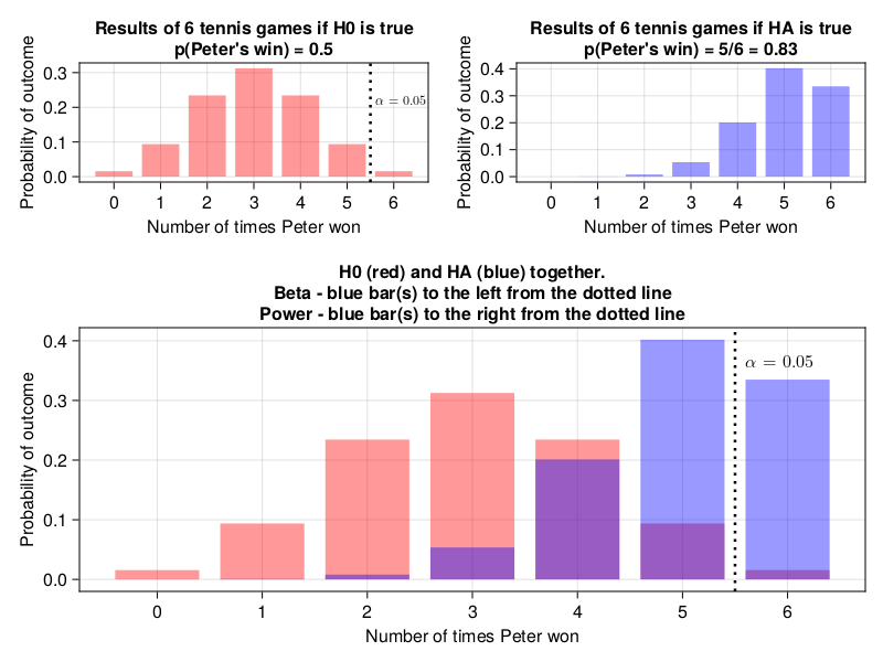
Figure 10: Graphical representation of the estimation process for type II error and the power of a test.

The top panels display the probability distributions for our experiment (6 games of tennis) under \(H_{0}\) (red bars) and \(H_{A}\) (blue bars). Notice, that the blue bars for 0, 1, and 2 are so small that they are barely (or not at all) visible on the graph. The black dotted vertical line is a cutoff level for type I error (or \(\alpha\)), which is 0.05. The bottom panel contains the distributions superimposed one on the other. The probability of type II error (or \(\beta\)) is the sum of the heights of the blue bar(s) to the left from the black dotted vertical line (the cutoff level for type I error). The power of a test is the sum of the heights of the blue bar(s) to the right from the black dotted vertical line (the cutoff level for type I error).

Hopefully the explanations above were clear enough. Still, the presented solution got a few flaws, i.e. we hard coded 6 into our functions (e.g. getResultOf1TennisGameUnderHA, play6tennisGamesGetPvalue), moreover running 100_000 simulations is probably less efficient than running purely mathematical calculations. Let’s try to add some plasticity and efficiency to our code (plus let’s check the accuracy of our computer simulation).

# to the right from that point on x-axis (>point) we reject H0 and choose HA
# n - number of trials (games)
function getXForBinomRightTailProb(n::Int, probH0::Float64,
                                   rightTailProb::Float64)::Int
    @assert (0 <= rightTailProb <= 1) "rightTailProb must be in range [0-1]"
    @assert (0 <= probH0 <= 1) "probH0 must be in range [0-1]"
    @assert (n > 0) "n must be positive"
    return Dsts.cquantile(Dsts.Binomial(n, probH0), rightTailProb)
end

# n - number of trials (games), x - number of successes (Peter's wins)
# returns probability (under HA) from far left up to (and including) x
function getBetaForBinomialHA(n::Int, x::Int, probHA::Float64)::Float64
    @assert (0 <= probHA <= 1) "probHA must be in range [0-1]"
    @assert (n > 0) "n must be positive"
    @assert (x >= 0) "x mustn't be negative"
    return Dsts.cdf(Dsts.Binomial(n, probHA), x)
end

Note: The above functions should work correctly if probH0 < probHA, i.e. the probability distribution under \(H_{0}\) is on the left and the probability distribution under \(H_{A}\) is on the right side of a graph, i.e. the case you see in Figure 10.

The function getXForBinomRightTailProb returns a value (number of Peter’s wins, number of successes, value on x-axis in Figure 10) above which we reject \(H_{0}\) in favor of \(H_{A}\) (if we feed it with cutoff for \(\alpha\) equal to 0.05). Take a look at Figure 10, it returns the value on x-axis to the right of which the sum of heights of the red bars is lower than the cutoff level for alpha (type I error). It does so by wrapping around Dsts.cquantile function (that runs the necessary mathematical calculations) for us.

Once we get this cutoff point (number of successes, here number of Peter’s wins) we can feed it as an input to getBetaForBinomialHA. Again, take a look at Figure 10, it calculates for us the sum of the heights of the blue bars from the far left (0 on x-axis) up-to the previously obtained cutoff point (the height of that bar is also included). Let’s see how it works in practice.

xCutoff = getXForBinomRightTailProb(6, 0.5, 0.05)
probOfType2error2 = getBetaForBinomialHA(6, xCutoff, 5/6)
powerOfTest2 = getPower(probOfType2error2)

(probOfType2error, probOfType2error2, powerOfTest, powerOfTest2)

(0.66384, 0.6651020233196159, 0.33616, 0.3348979766803841)

They appear to be close enough which indicates that our calculations with the computer simulation were correct.

Bonus. Sample size estimation.

As a bonus to this exercise let’s talk about sample sizes.

Notice that after solving this exercise we said that if Peter is actually a better player than John and wins on average 5:1 with his opponent then still, most likely we will not be able to show this with 6 tennis games (powerOfTest2 = 0.3349). So, if ten such experiments would be conducted around the world for similar Peters and Johns then roughly only in three of them Peter would be declared a better player after running statistical tests. That doesn’t sound right.

In order to overcome this at the onset of their experiment a statistician should also try to determine the proper sample size. First, he starts by asking himself a question: “how big difference will make a difference”. This is an arbitrary decision (at least a bit). Still, I think we can all agree that if Peter would win with John on average 99:1 then this would make a practical difference (probably John would not like to play with him, what’s the point if he would be still loosing). OK, and how about Peter wins with John on average 51:49. This does not make a practical difference. Here they are pretty well matched and would play with each other since it would be challenging enough for both of them and each one could win a decent amount of games to remain satisfied. Most likely, they would be even unaware of such a small difference.

In real life a physician could say, e.g. “I’m going to test a new drug that should reduce the level of ‘bad cholesterol’ (LDL-C). How big reduction would I like to detect? Hmm, I know, 30 [mg/dL] or more because it reduces the risk of a heart attack by 50%” or “By at least 25 [mg/dL] because the drug that is already on the market reduces it by 25 [mg/dL]” (the numbers were made up by me, I’m not a physician).

Anyway, once a statistician gets the difference that makes a difference he tries to estimate the sample size by making some reasonable assumptions about rest of the parameters.

In our tennis example we could write the following function for sample size estimation

# checks sample sizes between start and finish (inclusive, inclusive)
# assumes that probH0 is 0.5
function getSampleSizeBinomial(probHA::Float64,
    cutoffBeta::Float64=0.2,
    cutoffAlpha::Float64=0.05,
    twoTail::Bool=true,
    start::Int=6, finish::Int=40)::Int

    # other probs are asserted in the component functions that use them
    @assert (0 <= cutoffBeta <= 1) "cutoffBeta must be in range [0-1]"
    @assert (start > 0 && finish > 0) "start and finish must be positive"
    @assert (start < finish) "start must be smaller than finish"

    probH0::Float64 = 0.5
    sampleSize::Int = -99
    xCutoffForAlpha::Int = 0
    beta::Float64 = 1.0

    if probH0 >= probHA
        probHA = 1 - probHA
    end
    if twoTail
        cutoffAlpha = cutoffAlpha / 2
    end

    for n in start:finish
        xCutoffForAlpha = getXForBinomRightTailProb(n, probH0, cutoffAlpha)
        beta = getBetaForBinomialHA(n, xCutoffForAlpha, probHA)
        if beta <= cutoffBeta
            sampleSize = n
            break
        end
    end

    return sampleSize
end

Maybe that is not the most efficient method, but it should do the trick.

First, we initialize a few variables that we will use later (probH0, sampleSize, xCutoffForAlpha, beta). Then we compare probH0 with probHA. We do this since getXForBinomRightTailProb and getBetaForBinomialHA should work correctly only when probH0 < probHA (see the note under the code snippet with the functions definitions). Therefore we need to deal with the case when it is otherwise (if probH0 >= probHA). We do this by subtracting probHA from 1 and making it our new probHA (probHA = 1 - probHA). Because of that if we ever type, e.g. probHA = 1/6 = 0.166, then the function will transform it to probHA = 1 - 1/6 = 5/6 = 0.833 (since in our case the sample size required to demonstrate that Peter wins on average 1 out of 6 games, is the same as the sample size required to show that John wins on average 5 out of 6 games).

Once we are done with that we go to another checkup. If we are interested in two-tailed probability (twoTail) then we divide the number (cutoffAlpha = 0.05) by two. Before 0.05 went to the right side (see the black dotted line in Figure 10), now we split it, 0.025 goes to the left side, 0.025 goes to the right side of the probability distribution. This makes sense since before (see Section 4.7.4) we multiplied one-tailed probability by 2 to get the two-tailed probability, here we do the opposite. We can do that because the probability distribution under \(H_{0}\) (see the upper left panel in Figure 10) is symmetrical (that is why you mustn’t change the value of probH0 in the body of getSampleSizeBinomial).

Finally, we use the previously defined functions (getXForBinomRightTailProb and getBetaForBinomialHA) and conduct a series of experiments for different sample sizes (between start and finish). Once the obtained beta fulfills the requirement (beta <= cutoffBeta) we set sampleSize to that value (sampleSize = n) and stop subsequent search with a break statement (so if sampleSize of 6 is OK, we will not look at larger sample sizes). If the for loop terminates without satisfying our requirements then the value of -99 (sampleSize was initialized with it) is returned. This is an impossible value for a sample size. Therefore it points out that the search failed. Let’s put it to the test.

In this exercise we said that Peter wins with John on average 5:1 (\(H_{A}\), prob = 5/6 = 0.83). So what is the sample size necessary to confirm that with the acceptable type I error (\(alpha \le 0.05\)) and type II error (\(\beta \le 0.2\)) cutoffs.

# for one-tailed test
sampleSizeHA5to1 = getSampleSizeBinomial(5/6, 0.2, 0.05, false)
sampleSizeHA5to1

OK, so in order to be able to detect such a big difference (5:1, or even bigger) between the two tennis players they would have to play 13 games with each other (for one-tailed test). To put it into perspective and compare it with Figure 10 look at the graph below.

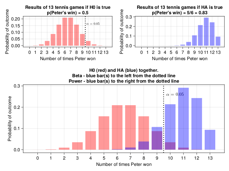
Figure 11: Graphical representation of type II error and the power of a test for 13 tennis games between Peter and John.

If our function worked well then the sum of the heights of the blue bars to the right of the black dotted line should be \(\ge 0.8\) (power of the test) and to the left should be \(\le 0.2\) (type II error or \(\beta\)).

(
    # alternative to the line below:
    # 1 - Dsts.cdf(Dsts.Binomial(13, 5/6), 9),
    Dsts.pdf.(Dsts.Binomial(13, 5/6), 10:13) |> sum,
    Dsts.cdf(Dsts.Binomial(13, 5/6), 9)
)

(0.841922621916511, 0.15807737808348934)

Yep, that’s correct. So, under those assumptions in order to confirm that Peter is a better tennis player he would have to win \(\ge 10\) games out of 13.

And how about the two-tailed probability (we expect the number of games to be greater).

# for two-tailed test
getSampleSizeBinomial(5/6, 0.2, 0.05)

Here we need 17 games to be sufficiently sure we can prove Peter’s supremacy.

OK. Let’s give our getSampleSizeBinomial one more swing. How about if Peter wins with John on average 4:2 (\(H_{A}\))?

# for two-tailed test
sampleSizeHA4to2 = getSampleSizeBinomial(4/6, 0.2, 0.05)
sampleSizeHA4to2

-99

Hmm, -99, so it will take more than 40 games (finish::Int = 40). Now, we can either stop here (since playing 40 games in a row is too time and energy consuming so we resign) or increase the value for finish like so

# for two-tailed test
sampleSizeHA4to2 = getSampleSizeBinomial(4/6, 0.2, 0.05, true, 6, 100)
sampleSizeHA4to2

Wow, if Peter is better than John in tennis and on average wins 4:2 then it would take 72 games to be sufficiently sure to prove it (who would have thought).

Anyway, if you ever find yourself in need to determine sample size, \(\beta\) or the power of a test (not only for one-sided tests as we did here) then you should probably consider using PowerAnalyses.jl which is on MIT license.

OK, I think you deserve some rest before moving to the next chapter so why won’t you take it now.

4.8 Statistics intro - Exerc.. ← → 5 Comparisons - continuous d..

CC BY-NC-SA 4.0 Bartlomiej Lukaszuk