7.9 Solutions - Association

In this sub-chapter you will find exemplary solutions to the exercises from the previous section.

7.9.1 Solution to Exercise 1

Let’s write getRanks, but let’s start simple and use it on a sorted vector [100, 500, 1000] without ties. In this case the body of getRanks function would be something like.

# for now the function is without types
function getRanksVer1(v)
    # or: ranks = collect(1:length(v))
    ranks = collect(eachindex(v))
    return ranks
end

getRanksVer1([100, 500, 1000])

[1, 2, 3]

Time to complicate stuff a bit by adding some ties in numbers.

# for now the function is without types
function getRanksVer2(v)
    initialRanks = collect(eachindex(v))
    finalRanks = zeros(length(v))
    for i in eachindex(v)
        indicesInV = findall(x -> x == v[i], v)
        finalRanks[i] = Stats.mean(initialRanks[indicesInV])
    end
    return finalRanks
end

(
    getRanksVer2([100, 500, 500, 1000]),
    getRanksVer2([100, 500, 500, 500, 1000])
)

([1.0, 2.5, 2.5, 4.0],
 [1.0, 3.0, 3.0, 3.0, 5.0])

The findall function accepts a function (here x -> x == v[i]) and a vector (here v). Next, it runs the function on every element of the vector and returns the indices for which the result was true. Here we are looking for elements in v that are equal to the currently examined (v[i]) element of v. Then, we use indicesInV to get the initialRanks. The initialRanks[indicesInV] returns a Vector that contains one or more (if ties occur) initialRanks for a given element of v. Finally, we calculate the average rank for a given number in v by using Stats.mean. The function may be sub-optimall as for [100, 500, 500, 1000] the average rank for 500 is calculated twice (once for 500 at index 2 and once for 500 at index 3) and for [100, 500, 500, 500, 1000] the average rank for 500 is calculated three times. Still, we are more concerned with the correct result and not the efficiency (assuming that the function is fast enough) so we will leave it as it is.

Now, the final tweak. The input vector is shuffled.

# for now the function is without types
function getRanksVer3(v)
    sortedV = collect(sort(v))
    initialRanks = collect(eachindex(sortedV))
    finalRanks = zeros(length(v))
    for i in eachindex(v)
        indicesInSortedV = findall(x -> x == v[i], sortedV)
        finalRanks[i] = Stats.mean(initialRanks[indicesInSortedV])
    end
    return finalRanks
end

(
    getRanksVer3([500, 100, 1000]),
    getRanksVer3([500, 100, 500, 1000]),
    getRanksVer3([500, 100, 500, 1000, 500])
)

([2.0, 1.0, 3.0],
 [2.5, 1.0, 2.5, 4.0],
 [3.0, 1.0, 3.0, 5.0, 3.0])

Here, we let the built in function sort to arrange the numbers from v in the ascending order. Then for each number from v we get its indices in sortedV and their corresponding ranks based on that (initialRanks[indicesInSortedV]). As in getRanksVer2 the latter is used to calculate their average.

OK, time for cleanup + adding some types for future references (before we forget them).

function getRanks(v::Vector{<:Real})::Vector{<:Float64}
    sortedV::Vector{<:Real} = collect(sort(v))
    initialRanks::Vector{<:Int} = collect(eachindex(sortedV))
    finalRanks::Vector{<:Float64} = zeros(length(v))
    for i in eachindex(v)
        indicesInSortedV = findall(x -> x == v[i], sortedV)
        finalRanks[i] = Stats.mean(initialRanks[indicesInSortedV])
    end
    return finalRanks
end

(
    getRanks([100, 500, 1000]),
    getRanks([100, 500, 500, 1000]),
    getRanks([500, 100, 1000]),
    getRanks([500, 100, 500, 1000]),
    getRanks([500, 100, 500, 1000, 500])
)

([1.0, 2.0, 3.0],
 [1.0, 2.5, 2.5, 4.0],
 [2.0, 1.0, 3.0],
 [2.5, 1.0, 2.5, 4.0],
 [3.0, 1.0, 3.0, 5.0, 3.0])

At long last we can define getSpearmCorAndPval and apply it to animals data frame.

function getSpearmCorAndPval(
    v1::Vector{<:Real}, v2::Vector{<:Real})::Tuple{Float64, Float64}
    return getCorAndPval(getRanks(v1), getRanks(v2))
end

getSpearmCorAndPval(animals.Body, animals.Brain)

(0.7162994456021085, 1.8128636948722132e-5)

The result appears to reflect the general relationship well (compare with Figure 34).

7.9.2 Solution to Exercise 2

The solution should be quite simple assuming you did solve exercise 4 from ch05 (see Section 5.7.4 and Section 5.8.4) and exercise 5 from ch06 (see Section 6.7.5 and Section 6.8.5).

Let’s start with the helper functions, getUniquePairs (Section 5.8.4) and getSortedKeysVals (Section 4.5) that we developed previously. For your convenience I paste them below.

function getUniquePairs(names::Vector{T})::Vector{Tuple{T,T}} where T
    @assert (length(names) >= 2) "the input must be of length >= 2"
    uniquePairs::Vector{Tuple{T,T}} =
        Vector{Tuple{T,T}}(undef, binomial(length(names), 2))
    currInd::Int = 1
    for i in eachindex(names)[1:(end-1)]
        for j in eachindex(names)[(i+1):end]
            uniquePairs[currInd] = (names[i], names[j])
            currInd += 1
        end
    end
    return uniquePairs
end

function getSortedKeysVals(d::Dict{T1,T2})::Tuple{
    Vector{T1},Vector{T2}} where {T1,T2}
    sortedKeys::Vector{T1} = keys(d) |> collect |> sort
    sortedVals::Vector{T2} = [d[k] for k in sortedKeys]
    return (sortedKeys, sortedVals)
end

Now, time to get all possible ‘raw’ correlations.

function getAllCorsAndPvals(
    df::Dfs.DataFrame, colsNames::Vector{String}
)::Dict{Tuple{String,String},Tuple{Float64,Float64}}

    uniquePairs::Vector{Tuple{String,String}} = getUniquePairs(colsNames)
    allCors::Dict{Tuple{String,String},Tuple{Float64,Float64}} = Dict(
        (n1, n2) => getCorAndPval(df[!, n1], df[!, n2]) for (n1, n2)
        in
        uniquePairs)

    return allCors
end

getAllCorsAndPvals (generic function with 1 method)

We start by getting the uniquePairs for the columns of interest colNames. Then we use dictionary comprehension to get our result. We iterate through each pair for (n1, n2) in uniquePairs. Each uniquePair is composed of a tuple (n1, n2), where n1 - name1, n2 - name2. While traversing the uniquePairs we calculate the correlations and p-values (getCorAndPval) by selecting columns of interest (df[:, n1] and df[:, n2]). And that’s it. Let’s see how it works and how many false positives we got (remember, we expect 2 or 3).

allCorsPvals = getAllCorsAndPvals(bogusCors, letters)
falsePositves = (map(t -> t[2], values(allCorsPvals)) .<= 0.05) |> sum
falsePositves

3

First, we extract the values from our dictionary with values(allCorsPvals). The values are a vector of tuples [(cor, pval)]. To get p-values alone, we use map function that takes every tuple (t) and returns its second element (t[2]). Finally, we compare the p-values with our cutoff level for type 1 error (\(\alpha = 0.05\)). And sum the Bools (each true is counted as 1, and each false as 0).

Anyway, as expected we got 3 false positives. All that’s left to do is to apply the multiplicity correction.

function adjustPvals(
    corsAndPvals::Dict{Tuple{String,String},Tuple{Float64,Float64}},
    adjMeth::Type{M}
)::Dict{Tuple{String,String},Tuple{Float64,Float64}} where
    {M<:Mt.PValueAdjustment}

    ks, vs = getSortedKeysVals(corsAndPvals)
    cors::Vector{<:Float64} = map(t -> t[1], vs)
    pvals::Vector{<:Float64} = map(t -> t[2], vs)
    adjustedPVals::Vector{<:Float64} = Mt.adjust(pvals, adjMeth())
    newVs::Vector{Tuple{Float64,Float64}} = collect(
        zip(cors, adjustedPVals))

    return Dict(ks[i] => newVs[i] for i in eachindex(ks))
end

adjustPvals (generic function with 1 method)

The code is rather self explanatory and relies on step by step operations: 1) getting our p-values (pvals), 2) applying an adjustment method (adjMeth) on them (Mt.adjust), and 3) combining the adjusted p-values (adjustedPVals) with cors again. For that last purpose we use zip function we met in Section 6.8.1. Finally we recreate a dictionary using comprehension. Time for some tests.

allCorsPvalsAdj = adjustPvals(allCorsPvals, Mt.BenjaminiHochberg)
falsePositves = (map(t -> t[2], values(allCorsPvalsAdj)) .<= 0.05) |> sum
falsePositves

0

We cannot expect a multiplicity correction to be a 100% error-proof solution. Still, it’s better than doing nothing and in our case it did the trick, we got rid of false positives.

7.9.3 Solution to Exercise 3

Let’s start by writing a function to get a correlation matrix. We could use for that Stats.cor like so Stats.cor(bogusCors). But since we need to add significance markers then the p-values for the correlations are indispensable. As far as I’m aware the package does not have it, then we will write a function of our own.

function getCorsAndPvalsMatrix(
    df::Dfs.DataFrame,
    colNames::Vector{String})::Array{<:Tuple{Float64, Float64}}

    len::Int = length(colNames)
    corsPvals::Dict{Tuple{String,String},Tuple{Float64,Float64}} =
        getAllCorsAndPvals(df, colNames)
    mCorsPvals::Array{Tuple{Float64,Float64}} = fill((0.0, 0.0), len, len)

    for cn in eachindex(colNames) # cn - column number
        for rn in eachindex(colNames) # rn - row number
            corPval = (
                haskey(corsPvals, (colNames[rn], colNames[cn])) ?
                corsPvals[(colNames[rn], colNames[cn])] :
                get(corsPvals, (colNames[cn], colNames[rn]), (1, 1))
            )
            mCorsPvals[rn, cn] = corPval
        end
    end

    return mCorsPvals
end

getCorsAndPvalsMatrix (generic function with 1 method)

The function getCorsAndPvalsMatrix uses getAllCorsAndPvals we developed previously (Section 7.9.2). Then we define the matrix (our result), we initialize it with the fill function that takes an initial value and returns an array of a given size filled with that value ((0.0, 0.0)). Next, we replace the initial values in mCorsPvals with the correct ones by using two for loops. Inside them we extract a tuple (corPval) from the unique corsPvals. First, we test if a corPval for a given two variables (e.g. “a” and “b”) is in the dictionary corsPvals (haskey etc.). If so then we insert it into the mCorsPvals. If not, then we search in corsPvals by its reverse (so, e.g. “b” and “a”) with get(corsPvals, (colNames[cn], colNames[rn]), etc.). If that combination is not present then we are looking for the correlation of a variable with itself (e.g. “a” and “a”) which is equal to (1, 1) (for correlation coefficient and p-value, respectively). Once we are done we return our mCorsPvals matrix (aka Array). Time to give it a test run.

getCorsAndPvalsMatrix(bogusCors, ["a", "b", "c"])

3×3 Matrix{Tuple{Float64, Float64}}:
 (1.0, 1.0)             (0.194, 0.591239)      (-0.432251, 0.212195)
 (0.194, 0.591239)      (1.0, 1.0)             (-0.205942, 0.568128)
 (-0.432251, 0.212195)  (-0.205942, 0.568128)  (1.0, 1.0)

The numbers seem to be OK. In the future, you may consider changing the function so that the p-values are adjusted, e.g. by using Mt.BenjaminiHochberg correction, but here we need some statistical significance for our heatmap so we will leave it as it is.

Now, let’s move to drawing a plot.

mCorsPvals = getCorsAndPvalsMatrix(bogusCors, letters)
cors = map(t -> t[1], mCorsPvals)
pvals = map(t -> t[2], mCorsPvals)
nRows, _ = size(cors) # same num of rows and cols in our matrix
xs = repeat(1:nRows, inner=nRows)
ys = repeat(1:nRows, outer=nRows)[end:-1:1]

fig = Cmk.Figure()
ax, hm = Cmk.heatmap(fig[1, 1], xs, ys, [cors...],
    colormap=:RdBu, colorrange=(-1, 1),
    axis=(;
        xticks=(1:1:nRows, letters[1:nRows]),
        yticks=(1:1:nRows, letters[1:nRows][end:-1:1])
    ))
Cmk.hlines!(fig[1, 1], 1.5:1:nRows, color="black", linewidth=0.25)
Cmk.vlines!(fig[1, 1], 1.5:1:nRows, color="black", linewidth=0.25)
Cmk.Colorbar(fig[:, end+1], hm)
fig

We begin by preparing the necessary helper variables (mCorsPvals, cors, pvals, nRows, xs, ys). The last two are the coordinates of the centers of squares on the X- and Y-axis. The cors will be flattened row by row using [cors...] syntax. For your information repeat([1, 2], inner = 2) returns [1, 1, 2, 2] and repeat([1, 2], outer = 2) returns [1, 2, 1, 2]. The ys vector is then reversed with [end:-1:1] to make it reflect better the order of correlations in cors (left to right, row by row). The same goes for yticks below. The above was determined to be the right option by trial and error. The next important parameter is colorrange=(-1, 1) it ensures that -1 is always the leftmost color (red) from the :RdBu colormap and 1 is always the rightmost color (blue) from the colormap. Without it the colors would be set to minimum(cors) and maximum(cors) which we do not want since the minimum will change from matrix to matrix. Over our heatmap we overlay the grid (hlines! and vlines!) to make the squares separate better from each other. The centers of the squares are at integers, and the edges are at halves, that’s why we start the ticks at 1.5. Finally, we add Colorbar as they did in the docs for Cmk.heatmap. The result of this code is visible in Figure 33 from the previous section.

OK, let’s add the correlation coefficients and statistical significance markers. But first, two little helper functions.

function getColorForCor(corCoeff::Float64)::String
    @assert (0 <= abs(corCoeff) <= 1) "abc(corCoeff) must be in range [0-1]"
    return (abs(corCoeff) >= 0.65) ? "white" : "black"
end

function getMarkerForPval(pval::Float64)::String
    @assert (0 <= pval <= 1) "probability must be in range [0-1]"
    return (pval <= 0.05) ? "#" : ""
end

getMarkerForPval (generic function with 1 method)

As you can see getColorForCor returns a color (“white” or “black”) for a given value of correlation coefficient (white color will make it easier to read the correlation coefficient on a dark red/blue background of a square). On the other hand getMarkerForPval returns a marker (“#”) when a pvalue is below our customary cutoff level for type I error.

fig = Cmk.Figure()
ax, hm = Cmk.heatmap(fig[1, 1], xs, ys, [cors...],
    colormap=:RdBu, colorrange=(-1, 1),
    axis=(;
        xticks=(1:1:nRows, letters[1:nRows]),
        yticks=(1:1:nRows, letters[1:nRows][end:-1:1])
    ))
Cmk.text!(fig[1, 1], xs, ys,
    text=string.(round.([cors...], digits=2)) .*
        getMarkerForPval.([pvals...]),
    align=(:center, :center),
    color=getColorForCor.([cors...]))
Cmk.hlines!(fig[1, 1], 1.5:1:nRows, color="black", linewidth=0.25)
Cmk.vlines!(fig[1, 1], 1.5:1:nRows, color="black", linewidth=0.25)
Cmk.Colorbar(fig[:, end+1], hm)
fig

The only new element here is Cmk.text! function, but since we used it a couple of times throughout this book, then I will leave the explanation of how the code piece works to you. Anyway, the result is to be found below.

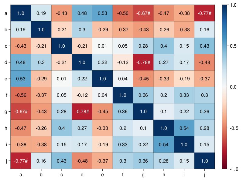
It looks good. Also the number of significance markers is right. Previously (Section 7.9.2) we said we got 3 significant correlations (based on ‘raw’ p-values). Since, the upper right triangle of the heatmap is a mirror reflection of the lower left triangle, then we should see 6 significance markers altogether. As a final step (that I leave to you) we could enclose the code from this task into a neat function named, e.g. drawHeatmap.

7.9.4 Solution to Exercise 4

OK, the code for this task is quite straightforward so let’s get right to it.

function drawDiagPlot(
    reg::Glm.StatsModels.TableRegressionModel,
    byCol::Bool = true)::Cmk.Figure
    dim::Vector{<:Int} = (byCol ? [1, 2] : [2, 1])
    res::Vector{<:Float64} = Glm.residuals(reg)
    pred::Vector{<:Float64} = Glm.predict(reg)
    form::String = string(Glm.formula(reg))
    fig = Cmk.Figure(size=(800, 800))
    Cmk.scatter(fig[1, 1], pred, res,
        axis=(;
            title="Residuals vs Fitted\n" * form,
            xlabel="Fitted values",
            ylabel="Residuals")
    )
    Cmk.hlines!(fig[1, 1], 0, linestyle=:dash, color="gray")
    Cmk.qqplot(fig[dim...],
        Dsts.Normal(0, 1),
        getZScore.(res, Stats.mean(res), Stats.std(res)),
        qqline=:identity,
        axis=(;
            title="Normal Q-Q\n" * form,
            xlabel="Theoretical Quantiles",
            ylabel="Standarized residuals")
    )
    return fig
end

We begin with extracting residuals (res) and predicted (pred) values from our model (reg). Additionally, we extract the formula (form) as a string. Then, we prepare a scatter plot (Cmk.scatter) with pred and res placed on X- and Y-axis, respectively. Next, we add a horizontal line (Cmk.hlines!) at 0 on Y-axis (the points should be randomly scattered around it). All that’s left to do is to build the required Q-Q plot (qqplot) with X-axis that contains the theoretical standard normal distribution (Dsts.Normal(0, 1)) and Y-axis with the standardized (getZScore) residuals (res). We also add qqline=:identity (here, identity means x = y) to facilitate the interpretation [if two distributions (on X- and Y-axis)] are alike then the points should lie roughly on the line. Since the visual impression we get may depend on the spacial arrangement (stretching or tightening of the points on a graph) our function enables us to choose (byCol) between column (true) and row (false) alignment of the subplots.

For a change let’s test our function on the iceMod2 from Section 7.7. Behold the result of drawDiagPlot(iceMod2, false).

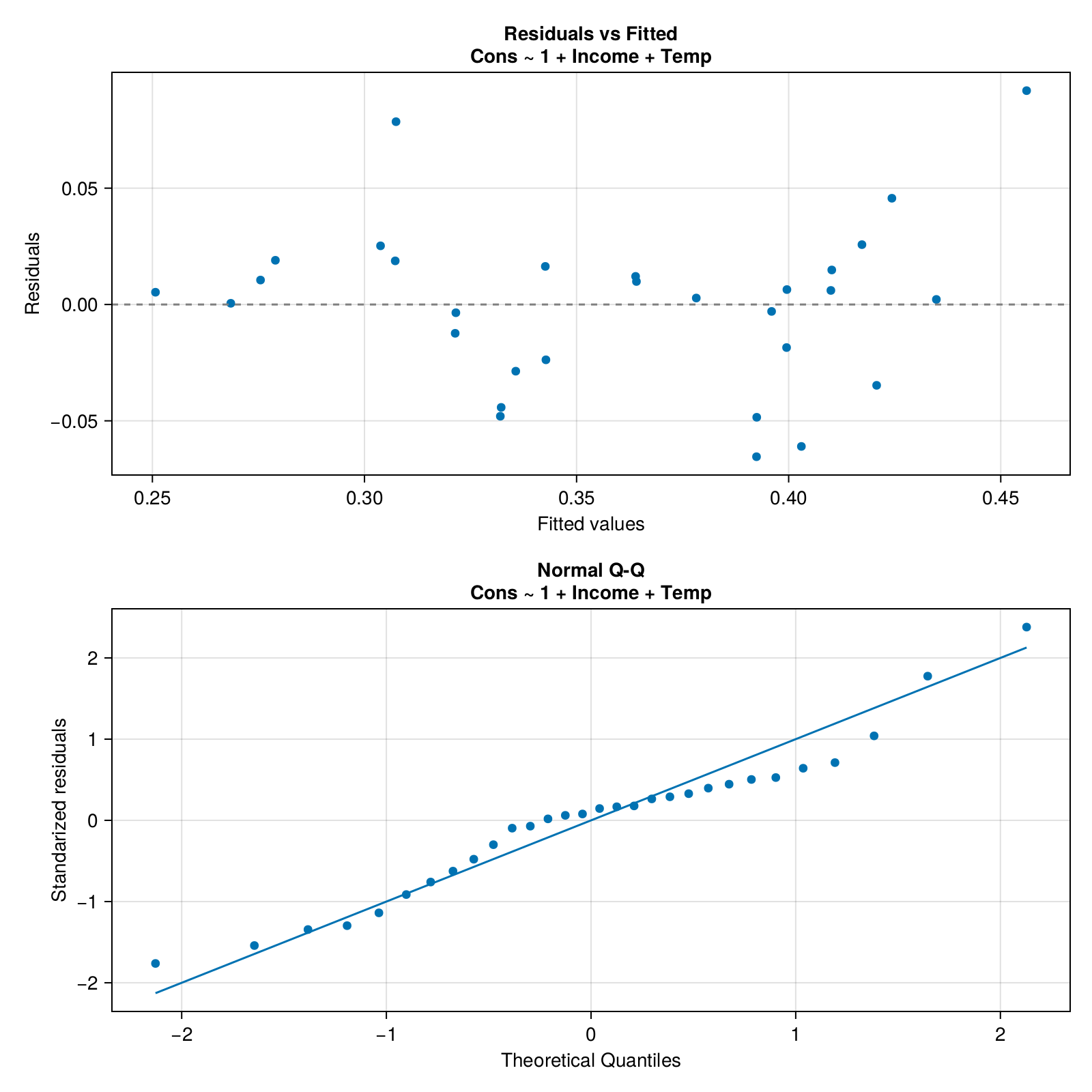
Hmm, I don’t know about you but to me the bottom panel looks rather normal. However, the top panel seems to display a wave (‘w’) pattern. This may be a sign of auto-correlation (explanation in a moment) and translate into instability of the estimation error produced by the model across the values of the explanatory variable(s). The error will display a wave pattern (once bigger once smaller). Now we got a choice, either we leave this model as it is (and we bear the consequences) or we try to find a better one.

To understand what the auto-correlation means in our case let’s do a thought experiment. Right now in the room that I am sitting the temperature is equal to 20 degrees of Celsius (68 deg. Fahrenheit). Which one is the more probable value of the temperature in 1 minute from now: 0 deg. Cels. (32 deg. Fahr.) or 21 deg. Cels. (70 deg. Fahr.)? I guess the latter is the more reasonable option. That is because the temperature one minute from now is a derivative of the temperature in the present (i.e. both values are correlated).

The same might be true for Icecream data frame, since it contains Temp column that we used in our model (iceMod2). We could try to remedy this by removing (kind of) the auto-correlation, e.g. with ice2 = ice[2:end, :] and ice2.TempDiff = ice.Temp[2:end] .- ice.Temp[1:(end-1)] and building our model a new. This is what we will do in the next exercise (although we will try to automate the process a bit).

7.9.5 Solution to Exercise 5

Let’s start with a few helper functions.

function getLinMod(
    df::Dfs.DataFrame,
    y::String, xs::Vector{<:String}
    )::Glm.StatsModels.TableRegressionModel
    return Glm.lm(Glm.term(y) ~ sum(Glm.term.(xs)), df)
end

function getPredictorsPvals(
    m::Glm.StatsModels.TableRegressionModel)::Vector{<:Float64}
    allPvals::Vector{<:Float64} = Glm.coeftable(m).cols[4]
    # 1st pvalue is for the intercept
    return allPvals[2:end]
end

function getIndsEltsNotEqlM(v::Vector{<:Real}, m::Real)::Vector{<:Int}
    return findall(x -> !isapprox(x, m), v)
end

We begin with getLinMod that accepts a data frame (df), name of the dependent variable (y) and names of the independent/predictor variables (xs). Based on the inputs it creates the model programmatically using Glm.term.

Next, we go with getPredictorsPvals that returns the p-values corresponding to a model’s coefficients.

Then, we define getIndsEltsNotEqlM that we will use to filter out the highest p-value from our model.

OK, time for the main actor of the show.

# returns minimal adequate (linear) model
function getMinAdeqMod(
    df::Dfs.DataFrame, y::String, xs::Vector{<:String}
    )::Glm.StatsModels.TableRegressionModel

    preds::Vector{<:String} = copy(xs)
    mod::Glm.StatsModels.TableRegressionModel = getLinMod(df, y, preds)
    pvals::Vector{<:Float64} = getPredictorsPvals(mod)
    maxPval::Float64 = maximum(pvals)
    inds::Vector{<:Int} = getIndsEltsNotEqlM(pvals, maxPval)

    for _ in xs
        if (maxPval <= 0.05)
            break
        end
        if (length(preds) == 1 && maxPval > 0.05)
            mod = Glm.lm(Glm.term(y) ~ Glm.term(1), df)
            break
        end
        preds = preds[inds]
        mod = getLinMod(df, y, preds)
        pvals = getPredictorsPvals(mod)
        maxPval = maximum(pvals)
        inds = getIndsEltsNotEqlM(pvals, maxPval)
    end

    return mod
end

We begin with defining the necessary variables that we will update in a for loop. The variables are: predictors (preds), linear model (mod), p-values for the model’s coefficients (pvals), maximum p-value (maxPval) and indices of predictors that we will leave in our model (inds). We start each iteration (for _ in xs) by checking if we already reached our minimal adequate model. To that end we make sure that all the remaining coefficients are statistically significant (if (maxPval <= 0.05)) or if we run out of the explanatory variables (length(preds) == 1 && maxPval > 0.05) we return our default (y ~ 1) model (the intercept of this model is equal to Stats.mean(y)). If not then we remove one predictor variable from the model (preds = preds[inds]) and update the remaining helper variables (mod, pvals, maxPval, inds). And that’s it, let’s see how it works.

ice2mod = getMinAdeqMod(ice2, names(ice2)[1], names(ice2)[2:end])
ice2mod

───────────────────────────────────────────────────────────────────────
               Coef.  Std. Error      t  Pr(>|t|)  Lower 95%  Upper 95%
───────────────────────────────────────────────────────────────────────
(Intercept)  -0.0672      0.0988  -0.68    0.5024    -0.2707     0.1363
Income        0.0031      0.001    2.99    0.0062     0.001      0.0053
Temp          0.0032      0.0004   7.99    <1e-99     0.0024     0.004
TempDiff      0.0022      0.0007   2.93    0.0071     0.0006     0.0037
───────────────────────────────────────────────────────────────────────

It appears to work as expected. Let’s compare it with a full model.

ice2FullMod = getLinMod(ice2, names(ice2)[1], names(ice2)[2:end])

Glm.ftest(ice2FullMod.model, ice2mod.model)

F-test: 2 models fitted on 29 observations
───────────────────────────────────────────────────────────────
     DOF  ΔDOF     SSR    ΔSSR      R²      ΔR²      F*   p(>F)
───────────────────────────────────────────────────────────────
[1]   10        0.0193          0.8450                         
[2]    5    -5  0.0227  0.0034  0.8179  -0.0272  0.7019  0.6285
───────────────────────────────────────────────────────────────

It looks good as well. We reduced the number of explanatory variables while maintaining comparable (p > 0.05) explanatory power of our model.

Time to check the assumptions with our diagnostic plot (drawDiagPlot from Section 7.9.1).

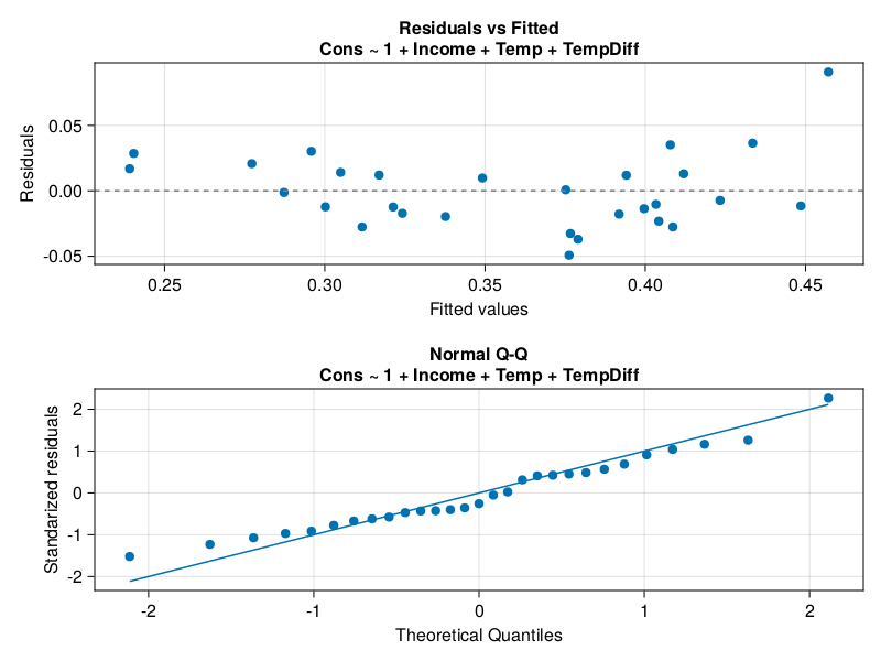
To me, the plot has slightly improved and since I run out of ideas how to make our model even better I’ll leave it as it is.

Now, let’s compare our ice2mod, that aimed to counteract the auto-correlation, with its predecessor (iceMod2). We will focus on the explanatory powers (adjusted \(r^2\), the higher the better)

(
    Glm.adjr2(iceMod2),
    Glm.adjr2(ice2mod)
)

(0.6799892012945553, 0.796000295561351)

and the average prediction errors (the lower the better).

(
    getAvgEstimError(iceMod2),
    getAvgEstimError(ice2mod)
)

(0.026114993652645798, 0.022116071809225545)

Again, it appears that we managed to improve our model’s prediction power at a cost of slightly more difficult interpretation (go ahead examine the output tables for Income + Temp + TempDiff vs. Income + Temp and explain to yourself how each variable influences the value of Cons). This is usually the case, the less straightforward the model, the less intuitive is its interpretation.

At a very long last we may check how our getMinAdeqMod will behave when there are no meaningful explanatory variables.

getMinAdeqMod(ice2, "Cons", ["a", "b", "c", "d"])

Cons ~ 1

Coefficients:
────────────────────────────────────────────────────────────────────────
                Coef.  Std. Error      t  Pr(>|t|)  Lower 95%  Upper 95%
────────────────────────────────────────────────────────────────────────
(Intercept)  0.358517    0.012397  28.92    <1e-21   0.333123   0.383911
────────────────────────────────────────────────────────────────────────

In that case (no meaningful explanatory variables) our best estimate (guess) of the value of y (here Cons) is the variable’s average (Stats.mean(ice2.Cons)) which is returned as the Coef. for (Intercept). In that case Std. Error is just the standard error of the mean that we met in Section 5.2 (compare with getSem(ice2.Cons)).

Anyway, building our minimal adequate model from top to bottom (as we did here) is not the only possible procedure. Equally reasonable is to apply the bottom to top approach. In that case we start with separate models with 1 explanatory variable each. Of those models we choose the one with the lowest p-value. Next we add to it one explanatory variable at a time (based on the p-value, the lower the better) until we reach our final model (no more significant explanatory variables left). Sadly, the two methods although equally sound do not always produce the same result (the same minimal adequate model). Unfortunately, as far as I’m aware there is not much to be done with it, so we must live with that fact.