5.8 Solutions - Comparisons of Continuous Data

In this sub-chapter you will find exemplary solutions to the exercises from the previous section.

5.8.1 Solution to Exercise 1

First the sample and the 100’000 simulations:

Rand.seed!(321)
ex1sample = Rand.rand(Dsts.Normal(80, 20), 10)
ex1sampleSd = Stats.std(ex1sample)
ex1sampleSem = getSem(ex1sample)
ex1sampleMeans = [
    Stats.mean(Rand.rand(Dsts.Normal(80, 20), 10))
    for _ in 1:100_000]
ex1sampleMeansMean = Stats.mean(ex1sampleMeans)
ex1sampleMeansSd = Stats.std(ex1sampleMeans)

The code doesn’t contain any new elements, so I will leave it to you to figure out what happened there.

And now, let’s move to the plot.

fig = Cmk.Figure()
Cmk.hist(fig[1, 1], ex1sampleMeans, bins=100, color=Cmk.RGBAf(0, 0, 1, 0.3),
    axis=(;
        title="Histogram of 100'000 sample means",
        xlabel="Adult human body weight [kg]",
        ylabel="Count"))
Cmk.ylims!(0, 4000)
Cmk.vlines!(fig[1, 1], 80,
    ymin=0.0, ymax=0.85, color="black", linestyle=:dashdot)
Cmk.text!(fig[1, 1], 81, 1000, text="population mean = 80")
Cmk.bracket!(fig[1, 1],
    ex1sampleMeansMean - ex1sampleMeansSd / 2, 3500,
    ex1sampleMeansMean + ex1sampleMeansSd / 2, 3500,
    style=:square
)
Cmk.text!(fig[1, 1], 72.5, 3700,
    text="sample means sd = 6.33")
Cmk.text!(fig[1, 1], 90, 3200,
    text="single sample sd = 17.32")
Cmk.text!(fig[1, 1], 90, 3000,
    text="single sample sem = 5.48")
fig

This produces the following graph.

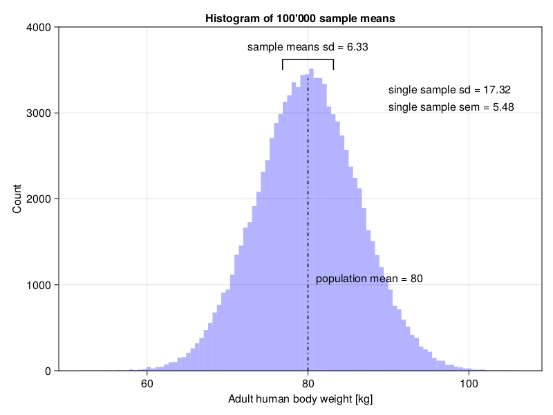
The graph clearly demonstrates that a better approximation of the samples means sd is a single sample sem and not a single sample sd (as stated in Section 5.2).

I’m not gonna explain the code snippet above in great detail since this is a warm up exercise, and the tutorials (e.g. the basic tutorial) and the documentation for the plotting functions (see the links in Section 5.7.1) are pretty good. Moreover, we already used CairoMakie plotting functions in Section 4.5. Still, a few quick notes are in order.

First of all, drawing a graph like that is not an enormous feat, you just need some knowledge (you read the tutorial and the function docs, right?). The rest is just patience and replication of the examples. Ah yes, I forgot about the try and error process [that happens from time to time (OK, more often than I would like to admit) in my case]. If an error happens, do not panic try to read the error’s message and think what it tells you).

It is always a good idea to annotate the graph, add the title, x- and y-axis labels (to make the reader’s, and your own, reasoning easier). Figures are developed from top to bottom (in the code), layer after layer (top line of code -> bottom layer on a graph, next line of code places a layer above the previous layer). First function (fig and Cmk.hist) creates the figure, the following functions (e.g. Cmk.text! and Cmk.vlines!), write/paint something on the previous layers. After some time and tweaking you should be able to produce quite pleasing figures (just remember, patience is the key). One more point, instead of typing strings by hand (like text="sample sd = 17.32") you may let Julia do that by using strings interpolation, like text="sample sd = $(round(ex1sampleSd, digits=2))"(with time you will appreciate the convenience of this method).

One more thing, the :dashdot (after the keyword argument linetype) is a Symbol. For now you may treat it like a string but written differently, i.e. :dashdot instead of "dashdot".

5.8.2 Solution to Exercise 2

First let’s start with the functions we developed in Section 4 (and its subsections). We already now them, so I will not explain them here.

function getCounts(v::Vector{T})::Dict{T,Int} where {T}
    counts::Dict{T,Int} = Dict()
    for elt in v
        counts[elt] = get(counts, elt, 0) + 1
    end
    return counts
end

function getProbs(counts::Dict{T,Int})::Dict{T,Float64} where {T}
    total::Int = sum(values(counts))
    return Dict(k => v / total for (k, v) in counts)
end

function getSortedKeysVals(d::Dict{A,B})::Tuple{
    Vector{A},Vector{B}} where {A,B}
    sortedKeys::Vector{A} = keys(d) |> collect |> sort
    sortedVals::Vector{B} = [d[k] for k in sortedKeys]
    return (sortedKeys, sortedVals)
end

Now, time to define getLstatistic based on what we learned in Section 5.4 (note, the function uses getAbsGroupDiffsAroundOverallMean and getAbsPointDiffsFromGroupMeans that we developed in that section).

function getLStatistic(v1::Vector{<:Real}, v2::Vector{<:Real})::Float64
    absDiffsOverallMean::Vector{<:Real} =
        getAbsGroupDiffsFromOverallMean(v1, v2)
    absDiffsGroupMean::Vector{<:Real} =
        getAbsPointDiffsFromGroupMeans(v1, v2)
    return Stats.mean(absDiffsOverallMean) / Stats.mean(absDiffsGroupMean)
end

OK, that was easy, after all we practically did it all before, we only needed to look for the components in the previous chapters. Now, the function to determine the distribution.

function getLStatisticsUnderH0(
    popMean::Real, popSd::Real,
    nPerGroup::Int=4, nIter::Int=1_000_000)::Vector{Float64}

    v1::Vector{Float64} = []
    v2::Vector{Float64} = []
    result::Vector{Float64} = zeros(nIter)

    for i in 1:nIter
        v1 = Rand.rand(Dsts.Normal(popMean, popSd), nPerGroup)
        v2 = Rand.rand(Dsts.Normal(popMean, popSd), nPerGroup)
        result[i] = getLStatistic(v1, v2)
    end

    return result
end

This one is slightly more complicated, so I think a bit of explanation is in order here. First we initialize some variables that we will use later. For instance, v1 and v2 will hold random samples drawn from a population of interest (Dsts.Normal(popMean, popSd)) and will change with each iteration. The vector result is initialized with 0s and will hold the LStatistic calculated during each iteration for v1 and v2. The result vector is returned by the function. Later on we will be able to use it to getCounts and getProbs for the L-Statistics. This should work just fine. However, if we slightly modify our function (getLStatisticsUnderH0), we could use it not only with the L-Statistic but also F-Statistic (optional points in this task) or any other statistic of interest. Observe

# getXStatFn signature: fnName(::Vector{<:Real}, ::Vector{<:Real})::Float64
function getXStatisticsUnderH0(
    getXStatFn::Function,
    popMean::Real, popSd::Real,
    nPerGroup::Int=4, nIter::Int=1_000_000)::Vector{Float64}

    v1::Vector{Float64} = []
    v2::Vector{Float64} = []
    result::Vector{Float64} = zeros(nIter)

    for i in 1:nIter
        v1 = Rand.rand(Dsts.Normal(popMean, popSd), nPerGroup)
        v2 = Rand.rand(Dsts.Normal(popMean, popSd), nPerGroup)
        result[i] = getXStatFn(v1, v2)
    end

    return result
end

Here, instead of getLStatisticsUnderH0 we named the function getXStatisticsUnderH0, where X is any statistic we can come up with. The function that calculates our statistic of interest is passed as a first argument to getXStatisticsUnderH0 (getXStatFn). The getXStatFn should work just fine, if it accepts two vectors (::Vector{<:Real}) and returns the statistic of interest (as Float64). Both those assumptions are fulfilled by getLStatistic (defined above) and getFStatistic defined in Section 5.4. To use our getXStatisticsUnderH0 we would type, e.g.: getXStatisticsUnderH0(getFStatistic, 25, 3, 4) or getXStatisticsUnderH0(getLStatistic, 25, 3, 4) instead of getLStatisticsUnderH0(25, 3, 4) that we defined in our first try (so more typing, but greater flexibility, and the result would be the same).

Now, to get a distribution of interest we use the following function

# getXStatFn signature: fnName(::Vector{<:Real}, ::Vector{<:Real})::Float64
function getXDistUnderH0(getXStatFn::Function,
    mean::Real, sd::Real,
    nPerGroup::Int=4, nIter::Int=10^6)::Dict{Float64,Float64}

    xStats::Vector{<:Float64} = getXStatisticsUnderH0(
        getXStatFn, mean, sd, nPerGroup, nIter)
    xStats = round.(xStats, digits=1)
    xCounts::Dict{Float64,Int} = getCounts(xStats)
    xProbs::Dict{Float64,Float64} = getProbs(xCounts)

    return xProbs
end

First, we calculate the statistics of interest (xStats), then we round the statistics to a 1 decimal point (round.(xStats, digits=1)). This is necessary, since in a moment we will use getCounts so we need some repetitions in our xStats vector (e.g. 1.283333331 and 1.283333332 will, both get rounded to 1.3 and the count for this value of the statistic will be 2). Once we got the counts, we change them to probabilities (fraction of times that the given value of the statistic occurred) with getProbs.

Now we can finally, use them to estimate the probability that the L-statistic greater than LStatisticEx2 = 1.28 occurred by chance.

Rand.seed!(321)
lprobs = getXDistUnderH0(getLStatistic, 25, 3)
lprobsGTLStatisticEx2 = [v for (k, v) in lprobs if k > LStatisticEx2]
lStatProb = sum(lprobsGTLStatisticEx2)

0.045378999999999996

Here, we used a comprehension with if. So, for every key-value pair ((k, v)) that is in lprobs we choose only those whose key (L-Statistic) is greater than LStatisticEx2 (if k > LStatisticEx2). In the last step we take only value ([v) from the pair (the value is the probability of such L-Statistic happening by chance alone) to our result lprobsGTLStatisticEx2. If this (comprehension with if) is to complicated for you then you may consider using filter and pipe (|>) the result to values |> collect.

The estimated probability for our L-Statistic is 0.045 which is pretty close to the probability obtained for the F-Statistic (Htests.OneWayANOVATest(ex2BwtsWater, ex2BwtsDrugY) |> Htests.pvalue = 0.043) (and well it should).

In virtually the same way we can get the experimental probability of an F-statistic being greater than getFStatistic(ex2BwtsWater, ex2BwtsDrugY) = 6.56 by chance. Observe

Rand.seed!(321)
cutoffFStat = getFStatistic(ex2BwtsWater, ex2BwtsDrugY)
fprobs = getXDistUnderH0(getFStatistic, 25, 3)
fprobsGTFStatisticEx2 = [v for (k, v) in fprobs if k > cutoffFStat]
fStatProb = sum(fprobsGTFStatisticEx2)

0.043154000000000005

Again, the p-value is quite similar to the one we got from a formal Htests.OneWayANOVATest (as it should be).

OK, now it’s time to draw some plots. First, let’s get the values for x- and y-axes

Rand.seed!(321)
# L distributions
lxs1, lys1 = getXDistUnderH0(getLStatistic, 25, 3) |> getSortedKeysVals
lxs2, lys2 = getXDistUnderH0(getLStatistic, 100, 50) |> getSortedKeysVals
lxs3, lys3 = getXDistUnderH0(getLStatistic, 25, 3, 8) |> getSortedKeysVals
# F distribution
fxs1, fys1 = getXDistUnderH0(getFStatistic, 25, 3) |> getSortedKeysVals

No, big deal L-Distributions start with l, the classical F-Distribution starts with f. BTW. Notice that thanks to getXDistUnderH0 we didn’t have to write two almost identical functions (getLDistUnderH0 and getFDistUnderH0).

OK, let’s place them on the graph

fig = Cmk.Figure()
ax1, l1 = Cmk.lines(fig[1, 1], fxs1, fys1, color="red",
    axis=(;
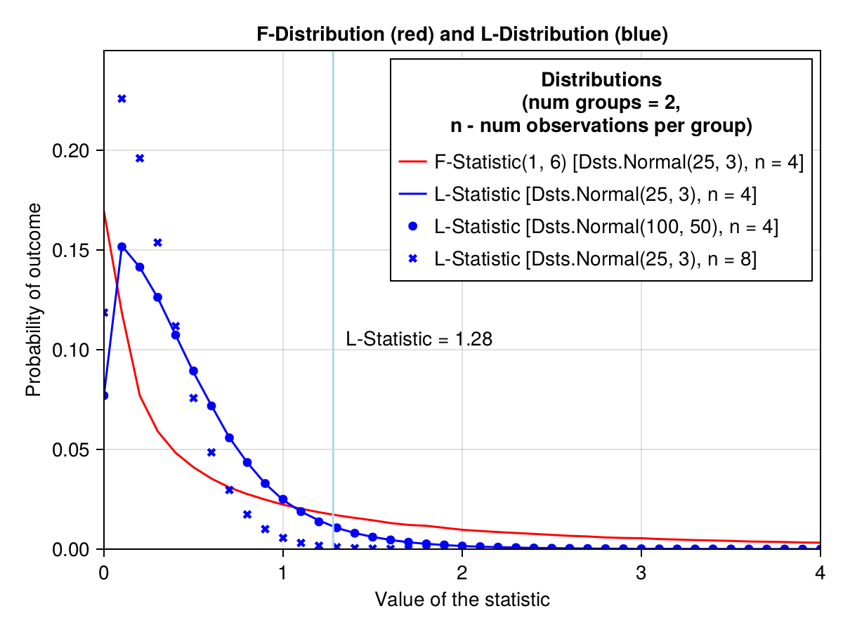
        title="F-Distribution (red) and L-Distribution (blue)",
        xlabel="Value of the statistic",
        ylabel="Probability of outcome"))
l2 = Cmk.lines!(fig[1, 1], lxs1, lys1, color="blue")
sc1 = Cmk.scatter!(fig[1, 1], lxs2, lys2, color="blue", marker=:circle)
sc2 = Cmk.scatter!(fig[1, 1], lxs3, lys3, color="blue", marker=:xcross)
Cmk.vlines!(fig[1, 1], LStatisticEx2, color="lightblue", type=:dashdot)
Cmk.text!(fig[1, 1], 1.35, 0.1,
    text="L-Statistic = 1.28")
Cmk.xlims!(0, 4)
Cmk.ylims!(0, 0.25)
Cmk.axislegend(ax1,
    [l1, l2, sc1, sc2],
    [
    "F-Statistic(1, 6) [Dsts.Normal(25, 3), n = 4]",
    "L-Statistic [Dsts.Normal(25, 3), n = 4]",
    "L-Statistic [Dsts.Normal(100, 50), n = 4]",
    "L-Statistic [Dsts.Normal(25, 3), n = 8]"
    ],
    "Distributions
(num groups = 2,
n - num observations per group)",
    position=:rt)
fig

Behold

Wow, what a beauty.

A few points of notice. Before, we calculated the probability (lStatProb) of getting the L-Statistic value greater than the vertical light blue line (the area under the blue curve to the right of that line). This is a one tail probability only. Interestingly, for the L-Distribution the mean and sd in the population of origin are not that important (blue circles for Dsts.Normal(100, 50) lie exactly on the blue line for Dsts.Normal(25, 3)). However, the number of groups and the number of observations per group affect the shape of the distribution (blue xcrosses for Dsts.Normal(25, 3) n = 8 diverge from the blue curve for Dsts.Normal(25, 3) n = 4).

The same is true for the F-Distribution. That is why the F-Distribution depends only on the degrees of freedom (Dsts.FDist(dfGroup, dfResidual)). The degrees of freedom depend on the number of groups and the number of observations per group.

5.8.3 Solution to Exercise 3

OK, let’s start with functions for checking the assumptions.

function areAllDistributionsNormal(vects::Vector{<:Vector{<:Real}})::Bool
    return [Pg.normality(v).pval[1] for v in vects] |>
        pvals -> map(pv -> pv > 0.05, pvals) |>
        all
end

function areAllVariancesEqual(vects::Vector{<:Vector{<:Real}})
    return Htests.FlignerKilleenTest(vects...) |>
        Htests.pvalue |> pv -> pv > 0.05
end

The functions above are basically just wrappers around the code we wrote in Section 5.5. Now, time for getPValUnpairedTest

function getPValUnpairedTest(
    v1::Vector{<:Real}, v2::Vector{<:Real})::Float64

    normality::Bool = areAllDistributionsNormal([v1, v2])
    homogeneity::Bool = areAllVariancesEqual([v1, v2])

    return (
        (normality && homogeneity) ? Htests.EqualVarianceTTest(v1, v2) :
        (normality) ? Htests.UnequalVarianceTTest(v1, v2) :
        Htests.MannWhitneyUTest(v1,v2)
        ) |> Htests.pvalue
end

The code is rather self-explanatory, of course if you remember the ternary expression from Section 3.5.2 and Section 3.9.4.

Let’s test our newly created function with the data from Section 5.3.2 (miceBwt)

getPValUnpairedTest([miceBwt[!, n] for n in Dfs.names(miceBwt)]...) |>
x -> round(x, digits=4)

0.0804

The p-value is the same as in Section 5.3.2 (as it should be), but this time we didn’t have to explicitly check the assumptions before applying the appropriate test.

5.8.4 Solution to Exercise 4

First, let’s start with a helper function that will return us all the possible pairs from a vector.

function getUniquePairs(uniqueNames::Vector{T})::Vector{Tuple{T,T}} where T

    @assert (length(uniqueNames) >= 2) "the input must be of length >= 2"

    uniquePairs::Vector{Tuple{T,T}} =
        Vector{Tuple{T,T}}(undef, binomial(length(uniqueNames), 2))
    currInd::Int = 1

    for i in eachindex(uniqueNames)[1:(end-1)]
        for j in eachindex(uniqueNames)[(i+1):end]
            uniquePairs[currInd] = (uniqueNames[i], uniqueNames[j])
            currInd += 1
        end
    end

    return uniquePairs
end

The function is generic, so it can be applied to vector of any type (T), here designed as Vector{T}. It starts by initializing an empty vector (uniquePairs) to hold the results. The initialization takes the following form: Vector{typeOfVectElements}(iniaialValues, lengthOfTheVector). The vector is filled with undefs (undefined values, some garbage) as placeholders. The size of the new vector is calculated by the binomial function. It is applied in the form binomial(n, k) where n is number of values to choose from and k is number of values per group. The function returns the number of possible groups of a given size. The rest is just iteration (for loops) over the indexes (eachindex) of the uniqueNames vector to get all the possible pairs. Let’s quickly check if the function works as expected.

(
    getUniquePairs([10, 20]),
    getUniquePairs([1.1, 2.2, 3.3]),
    getUniquePairs(["w", "x", "y", "z"]), # vector of one element Strings
    getUniquePairs(['a', 'b', 'c']), # vector of Chars
    getUniquePairs(['a', 'b', 'a']) # uniqueNames must be unique (of course)
)

([(10, 20)],
 [(1.1, 2.2), (1.1, 3.3), (2.2, 3.3)],
 [("w", "x"), ("w", "y"), ("w", "z"), ("x", "y"), ("x", "z"), ("y", "z")],
 [('a', 'b'), ('a', 'c'), ('b', 'c')],
 [('a', 'b'), ('a', 'a'), ('b', 'a')])

Note: The group (“w”, “x”) is the same group as (“x”, “w”). In other words, we don’t care about the order of elements in a group. The function works correctly if uniqueNames argument contains unique elements (compare with the last example that contains a duplicate value). If you want you can add an additional check to make sure that the uniqueNames are really unique (think/search the internet how to do that), but I will leave it as it is.

OK, now it’s time for getPValsUnpairedTests

# df - DataFrame: each column is a continuous variable (one group)
# returns uncorrected p-values
function getPValsUnpairedTests(
    df::Dfs.DataFrame)::Dict{Tuple{String,String},Float64}

    pairs::Vector{Tuple{String,String}} = getUniquePairs(Dfs.names(df))
    pvals::Vector{Float64} = [
        getPValUnpairedTest(df[!, a], df[!, b])
        for (a, b) in pairs
    ]

    return Dict(pairs[i] => pvals[i] for i in eachindex(pairs))
end

First, we obtain the pairs of group names that we will compare later (pairs). In the next few lines we use a comprehension to obtain the p-values. Since each element of pairs vector is a tuple (e.g. [("spA", "spB"), etc.]) we assign its elements to a and b (for (a, b)) and pass them to df to get the values of interest (e.g. df[!, a]). The values are send to getPValUnpairedTest from the previous section. We terminate (return) with another comprehension that creates a dictionary with the desired result.

Let’s see how the function works and compare the results with the ones we obtained in Section 5.5.

getPValsUnpairedTests(miceBwtABC)

Dict{Tuple{String, String}, Float64} with 3 entries:
  ("spA", "spB") => 0.0251115
  ("spA", "spC") => 0.000398545
  ("spB", "spC") => 0.0493322

OK, the uncorrected p-values are the same as in Section 5.5.

Now, the improved version.

# df - DataFrame: each column is a continuous variable (one group)
# returns corrected p-values
function getPValsUnpairedTests(
    df::Dfs.DataFrame,
    multCorr::Type{M}
)::Dict{Tuple{String,String},Float64} where {M<:Mt.PValueAdjustment}

    pairs::Vector{Tuple{String,String}} = getUniquePairs(Dfs.names(df))
    pvals::Vector{Float64} = [
        getPValUnpairedTest(df[!, a], df[!, b])
        for (a, b) in pairs
    ]
    pvals = Mt.adjust(pvals, multCorr())

    return Dict(pairs[i] => pvals[i] for i in eachindex(pairs))
end

Don’t worry about the strange type declarations like ::Type{M} and where {M<:Mt.PValueAdjustment}. I added them for the sake of consistency (after reading the code in the package repo and some try and error). When properly called, the function should work equally well without those parts.

Anyway, it wasn’t that bad, we basically just added a small piece of code (multCorr in the arguments list and pvals = Mt.adjust(pvals, multCorr()) in the function body) similar to the one in Section 5.6.

Let’s see how it works.

# Bonferroni correction
getPValsUnpairedTests(miceBwtABC, Mt.Bonferroni)

Dict{Tuple{String, String}, Float64} with 3 entries:
  ("spA", "spB") => 0.0753345
  ("spA", "spC") => 0.00119563
  ("spB", "spC") => 0.147997

That looks quite alright. Time for one more swing.

# Benjamini-Hochberg correction
getPValsUnpairedTests(miceBwtABC, Mt.BenjaminiHochberg)

Dict{Tuple{String, String}, Float64} with 3 entries:
  ("spA", "spB") => 0.0376673
  ("spA", "spC") => 0.00119563
  ("spB", "spC") => 0.0493322

Again, the p-values appear to be the same as those we saw in Section 5.6.

5.8.5 Solution to Exercise 5

OK, let’s do this step by step. First let’s draw a bare box-plot (no group names, no significance markers, titles, etc.).

The docs for Cmk.boxplot show that to do that we need two vectors for xs and ys (values to be placed on the x- and y-axis respectively). Both need to be of numeric types. We can achieve it by typing, e.g.

# Step 1
ex5nrows = size(miceBwtABC)[1] #1
ex5names = Dfs.names(miceBwtABC) #2
ex5xs = repeat(eachindex(ex5names), inner=ex5nrows) #3
ex5ys = [miceBwtABC[!, n] for n in ex5names] #4
ex5ys = vcat(ex5ys...) #5

Cmk.boxplot(ex5xs, ex5ys)

In the first line (#1) we get the dimensions of our data frame, size(miceBwtABC) returns a tuple (numberOfRows, numberOfColumns) from which we take only the first part (numberOfRows) that we will need later. In line 3 (#3) we assign a number to the names (eachindex(vect) returns a sequence 1:length(vect), e.g. [1, 2, 3]). We multiply each number the same amount of times (ex5nrows) using repeat (e.g. repeat([1, 2, 3], inner=2) returns [1, 1, 2, 2, 3, 3]). In line 4 and 5 (#4 and #5) we take all the body weights from columns and put them into a one long vector (ex5ys). We end up with two vectors: groups coded as integers and body weights. Finally, we check if it works by running Cmk.boxplot(ex5xs, ex5ys). The result is below.

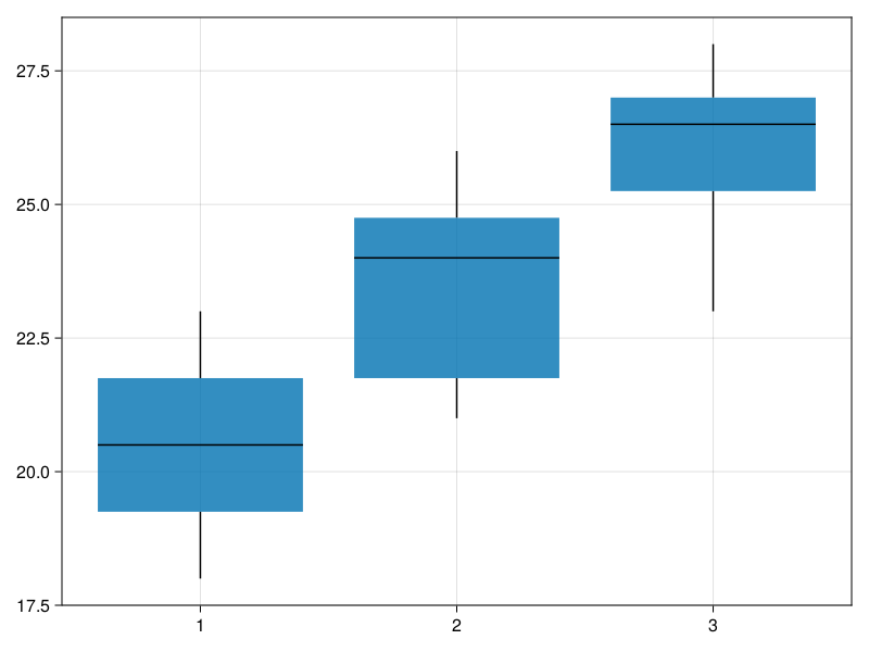
Now, let’s add title, label the axes, etc.

# Step 2
fig = Cmk.Figure()
Cmk.Axis(fig[1, 1], xticks=(eachindex(ex5names), ex5names),
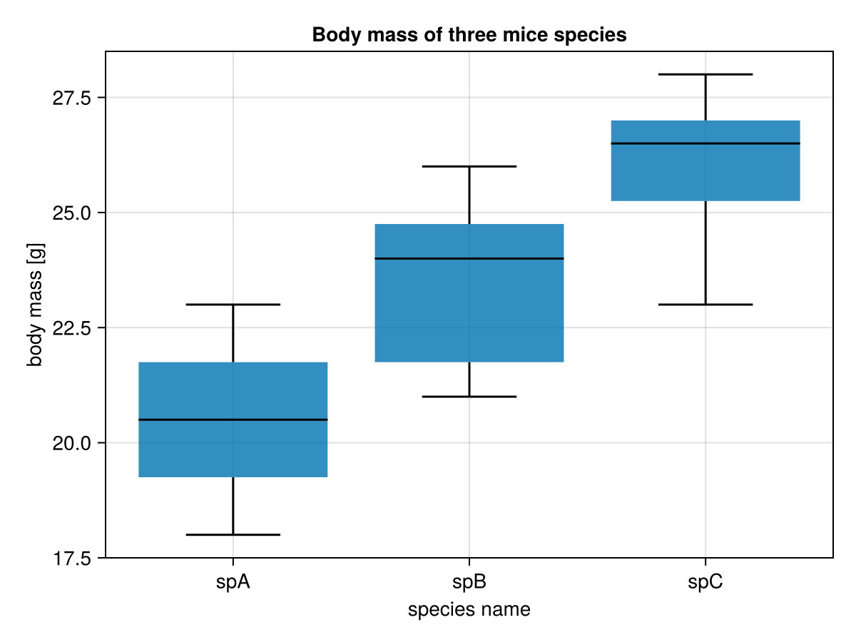
    title="Body mass of three mice species",
    xlabel="species name", ylabel="body mass [g]")
Cmk.boxplot!(fig[1, 1], ex5xs, ex5ys)
fig

The only new part here is the xticks argument. It takes a tuple of ticks on x axis (1:3 in Figure 20) and a vector of strings (ex5names) to be displayed instead of those values. The result is seen below.

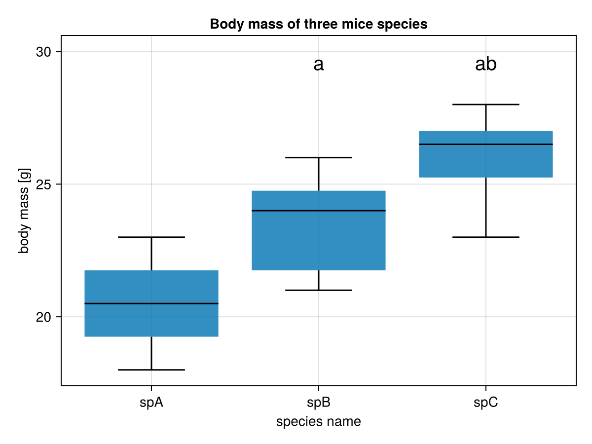
Let’s move on to the significance markers. First, let’s hard-code them and produce a plot (just to see if it works), then we will introduce some improvements.

# Step 3
fig = Cmk.Figure()
Cmk.Axis(fig[1, 1], xticks=(eachindex(ex5names), ex5names),
    title="Body mass of three mice species",
    xlabel="species name", ylabel="body mass [g]")
Cmk.boxplot!(fig[1, 1], ex5xs, ex5ys)
Cmk.text!(fig[1, 1],
    eachindex(ex5names), [30, 30, 30],
    text=["", "a", "ab"],
    align=(:center, :top), fontsize=20)
fig

OK, we’re almost there (see figure below).

However, it appears that we still need a few things:

1. a way to generate y-values for Cmk.text! (for now it is [30, 30, 30], but other dataframe may have different value ranges, e.g. [200-250] and then the markers would be placed too low)
2. a way to generate the markers (e.g. ["", "a", "ab"] based on p-values) over the appropriate boxes

The first problem can be solved in the following way:

# Step 4
ex5marksYpos = [maximum(miceBwtABC[!, n]) for n in ex5names] #1
ex5marksYpos = map(mYpos -> round(Int, mYpos * 1.1), ex5marksYpos) #2
ex5upYlim = maximum(ex5ys * 1.2) |> x -> round(Int, x) #3
ex5downYlim = minimum(ex5ys * 0.8) |> x -> round(Int, x) #4

Here, in the first line (#1) we get maximum values from every group. Then (#2) we increase them by 10% (* 1.1) and round them to the closest integers (round(Int,). At this height (y-axis) we are going to place our significance markers. Additionally, in lines 3 and 4 (#3 and #4) we found the maximum and minimum values (for all the data). We increase (* 1.2) and decrease (* 0.8) the values by 20%. The rounded (to the nearest integer) values will be the maximum and minimum values displayed on the y-axis of our graph.

Now, time for a function that will translate p-values to significance markers.

# Step 5
function getMarkers(
    pvs::Dict{Tuple{String,String},Float64},
    groupsOrder=["spA", "spB", "spC"],
    markerTypes::Vector{String}=["a", "b", "c"],
    cutoffAlpha::Float64=0.05)::Vector{String}

    @assert (
        length(groupsOrder) == length(markerTypes)
    ) "different groupsOrder and markerTypes lengths"
    @assert (0 <= cutoffAlpha <= 1) "cutoffAlpha must be in range [0-1]"

    markers::Vector{String} = repeat([""], length(groupsOrder))
    tmpInd::Int = 0

    for i in eachindex(groupsOrder)
        for ((g1, g2), pv) in pvs
            if (groupsOrder[i] == g1) && (pv <= cutoffAlpha)
                tmpInd = findfirst(x -> x == g2, groupsOrder)
                markers[tmpInd] *= markerTypes[i]
            end
        end
    end

    return markers
end

Here, getMarkers accepts p-values in the format returned by getPValsUnpairedTests defined in Section 5.8.4. Another input argument is groupsOrder which contains the position of groups (boxes, x-axis labels) in Figure 22 from left to right. The third argument is makrerTypes so a symbol that is to be used if a statistical difference for a given group is found.

The function defines markers (the strings placed over each box with Cmk.txt) initialized with a vector of empty strings. Next, it walks through each index in group (eachindex(groups)) and checks the ((g1, g2), pv) in p-values (pvs). If g1 is equal to the examined group (groups[i] == g1) and the p-value (pv) is \(\le\) the cutoff level then the appropriate marker (markerTypes[i]) is inserted by string concatenation with an update operator (*=). Which maker to change is determined by the index of g2 in the groups returned by findfirst function. In general, g2 receives a marker when it is statistically different from g1 (pv < cutoffAlpha).

Let’s test our function

(
getMarkers(
    getPValsUnpairedTests(miceBwtABC, Mt.BenjaminiHochberg),
    ["spA", "spB", "spC"],
    ["a", "b", "c"],
    0.05),

getPValsUnpairedTests(miceBwtABC, Mt.BenjaminiHochberg)
)

(["", "a", "ab"], 
Dict(("spA", "spB") => 0.0376672521079031,
("spA", "spC") => 0.001195633577293774,
("spB", "spC") => 0.049332195639921715))

The markers appear to be OK (they reflect the p-values well).

Now, it is time to pack it all into a separate function

# Step 6

# the function should work fine for up to 26 groups in the df's columns
function drawBoxplot(
    df::Dfs.DataFrame, title::String,
    xlabel::String, ylabel::String)::Cmk.Figure

    nrows, _ = size(df)
    ns::Vector{String} = Dfs.names(df)
    xs = repeat(eachindex(ns), inner=nrows)
    ys = [df[!, n] for n in ns]
    ys = vcat(ys...)
    marksYpos = [maximum(df[!, n]) for n in ns]
    marksYpos = map(mYpos -> round(Int, mYpos * 1.1), marksYpos)
    upYlim = maximum(ys * 1.2) |> x -> round(Int, x)
    downYlim = minimum(ys * 0.8) |> x -> round(Int, x)
    # 'a':'z' generates all lowercase chars of the alphabet
    markerTypes::Vector{String} = map(string, 'a':'z')
    markers::Vector{String} = getMarkers(
        getPValsUnpairedTests(df, Mt.BenjaminiHochberg),
        ns,
        markerTypes[1:length(ns)],
        0.05
    )

    fig = Cmk.Figure()
    Cmk.Axis(fig[1, 1], xticks=(eachindex(ns), ns),
        title=title,
        xlabel=xlabel, ylabel=ylabel)
    Cmk.boxplot!(fig[1, 1], xs, ys)
    Cmk.ylims!(downYlim, upYlim)
    Cmk.text!(fig[1, 1],
        eachindex(ns), marksYpos,
        text=markers,
        align=(:center, :top), fontsize=20)

    return fig
end

and run it

drawBoxplot(miceBwtABC,
    "Body mass of three mice species",
    "species name",
    "body mass [g]"
)

And voilà this is your result

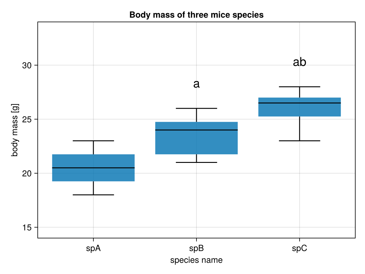
Once again (we said this already in the task description see Section 5.7.5). In the graph above a middle horizontal line in a box is the median, a box depicts interquartile range (IQR), the whiskers length is equal to 1.5 * IQR (or the maximum and minimum if they are smaller than 1.5 * IQR).

You could make the function more plastic, e.g. by moving some of its insides to its argument list. But this form will do for now. You may want to test the function with some other output, even with miceBwt from Section 5.3 (here it should draw a box-plot with no statistical significance markers).

Note: The code we developed in the exercises (e.g. getPValsUnpairedTests, drawBoxplot) is to help us automate stuff, still it shouldn’t be applied automatically (think before you leap).