7.7 Multiple Linear Regression
Multiple linear regression is a linear regression with more than one predictor variable. Take a look at the Icecream data frame.
ice = RD.dataset("Ecdat", "Icecream")
first(ice, 5)
| Cons | Income | Price | Temp |
|---|---|---|---|
| 0.386 | 78.0 | 0.27 | 41.0 |
| 0.374 | 79.0 | 0.282 | 56.0 |
| 0.393 | 81.0 | 0.277 | 63.0 |
| 0.425 | 80.0 | 0.28 | 68.0 |
| 0.406 | 76.0 | 0.272 | 69.0 |
We got 4 columns altogether (more detail in the link above):
Cons- consumption of ice cream (pints),Income- average family income per week (USD),Price- price of ice cream (USD per pint),Temp- temperature (Fahrenheit)
Imagine you are an ice cream truck owner and are interested to know which factors influence (and in what way) the consumption (Cons) of ice-cream by your customers. Let’s start by building a model with all the possible explanatory variables.
iceMod1 = Glm.lm(Glm.@formula(Cons ~ Income + Price + Temp), ice)
iceMod1
───────────────────────────────────────────────────────────────────────
               Coef.  Std. Error      t  Pr(>|t|)  Lower 95%  Upper 95%
───────────────────────────────────────────────────────────────────────
(Intercept)   0.1973      0.2702   0.73    0.4718    -0.3581     0.7528
Income        0.0033      0.0012   2.82    0.0090     0.0009     0.0057
Price        -1.0444      0.8344  -1.25    0.2218    -2.7595     0.6706
Temp          0.0035      0.0004   7.76    <1e-99     0.0025     0.0044
───────────────────────────────────────────────────────────────────────
Right away we can see that the price of ice-cream negatively affects (Coef. = -1.044) the volume of ice cream consumed (the more expensive the ice cream is the less people eat it, 1.044 pint less for every additional USD of price). The relationship is in line with our intuition. However, there is not enough evidence (p > 0.05) that the real influence of Price on consumption isn’t 0 (so no influence). Therefore, you wonder should you perhaps remove the variable Price from the model like so
iceMod2 = Glm.lm(Glm.@formula(Cons ~ Income + Temp), ice)
iceMod2
───────────────────────────────────────────────────────────────────────
               Coef.  Std. Error      t  Pr(>|t|)  Lower 95%  Upper 95%
───────────────────────────────────────────────────────────────────────
(Intercept)  -0.1132      0.1083  -1.05    0.3051    -0.3354     0.109
Income        0.0035      0.0012   3.02    0.0055     0.0011     0.0059
Temp          0.0035      0.0004   7.96    <1e-99     0.0026     0.0045
───────────────────────────────────────────────────────────────────────
Now, we got Income and Temp in our model, both of which are statistically significant. The values of Coef.s for Income and Temp somewhat changed between the models, but such changes (and even greater) are to be expected. Still, we would like to know if our new iceMod2 is really better than iceMod1 that we came up with before.
In our first try to solve the problem we could resort to the coefficient of determination (\(r^2\)) that we met in Section 7.6. Intuition tells us that a better model should have a bigger \(r^2\).
round.([Glm.r2(iceMod1), Glm.r2(iceMod2)],
    digits = 3)
[0.719, 0.702]Hmm, \(r^2\) is bigger for iceMod1 than iceMod2. However, there are two problems with it: 1) the difference between the coefficients is quite small, and 2) \(r^2\) gets easily inflated by any additional variable in the model. And I mean any, if you add, let’s say 10 random variables to the ice data frame and put them into a model the coefficient of determination will go up even though this makes no sense (we know their real influence is 0). That is why we got an improved metrics called the adjusted coefficient of determination. This parameter (adj. \(r^2\)) penalizes for every additional variable added to our model. Therefore the ‘noise’ variables will lower the adjusted \(r^2\) whereas only truly impactful ones will be able to raise it.
round.([Glm.adjr2(iceMod1), Glm.adjr2(iceMod2)],
    digits = 3)
[0.687, 0.68]iceMod1 still explains more variability in Cons (ice cream consumption), but the magnitude of the difference dropped. This makes our decision even harder. Luckily, Glm has ftest function to help us determine if one model is significantly better than the other.
Glm.ftest(iceMod1.model, iceMod2.model)F-test: 2 models fitted on 30 observations
───────────────────────────────────────────────────────────────
DOF ΔDOF SSR ΔSSR R² ΔR² F* p(>F)
───────────────────────────────────────────────────────────────
[1] 5 0.0353 0.7190
[2] 4 -1 0.0374 0.0021 0.7021 -0.0169 1.5669 0.2218
───────────────────────────────────────────────────────────────The table contains two rows:
[1]- first model from the left (inGlm.ftestargument list)[2]- second model from the left (inGlm.ftestargument list)
and a few columns:
DOF- degrees of freedom (more elements in formula, biggerDOF)ΔDOF-DOF[2]-DOF[1]SSR- residual sum of squares (the smaller the better)ΔSSR-SSR[2]-SSR[1]R2- coefficient of determination (the bigger the better)ΔR2-R2[2]-R2[1]F*- F-Statistic (similar to the one we met in Section 5.4)p(>F)- p-value that you obtain F-statistic greater than the one in the previous column by chance alone (assuming both models are equally good)
Based on the test we see that none of the models is clearly better than the other (p > 0.05). Therefore, in line with Occam’s razor principle (when two equally good explanations exist, choose the simpler one) we can safely pick iceMod2 as our final model.
What we did here was the construction of a so called minimal adequate model (the smallest model that explains the greatest amount of variance in the dependent/outcome variable). We did this using top to bottom approach. We started with a ‘full’ model. Then, we followed by removing explanatory variables (one by one) that do not contribute to the model (we start from the highest p-value above 0.05) until only meaningful explanatory variables remain. The removal of the variables reflects our common sense, because usually we (or others that will use our model) do not want to spend time/money/energy on collecting data that are of no use to us.
OK, let’s inspect our minimal adequate model again.
iceMod2
───────────────────────────────────────────────────────────────────────
               Coef.  Std. Error      t  Pr(>|t|)  Lower 95%  Upper 95%
───────────────────────────────────────────────────────────────────────
(Intercept)  -0.1132      0.1083  -1.05    0.3051    -0.3354     0.109
Income        0.0035      0.0012   3.02    0.0055     0.0011     0.0059
Temp          0.0035      0.0004   7.96    <1e-99     0.0026     0.0045
───────────────────────────────────────────────────────────────────────
We can see that for every extra dollar of Income our customers consume 0.003 pint (~1.47 mL) of ice cream more. Roughly the same change is produced by each additional grade (in Fahrenheit) of temperature. So, a simultaneous increase in Income by 1 USD and Temp by 1 unit translates into roughly 0.003 + 0.003 = 0.006 pint (~2.94 mL) greater consumption of ice cream per person. Now, (remember you were to imagine you are an ice cream truck owner) you could use the model to make predictions (with Glm.predict as we did in Section 7.6) to your benefit (e.g. by preparing enough product for your customers on a hot day).
So the time passes by and one sunny day when you open a bottle of beer a drunk genie pops out of it. To compensate you for the lost beer he offers to fulfill one wish (shouldn’t there be three?). He won’t shower you with cash right away since you will not be able to explain it to the tax office. Instead, he will give you the ability to control either Income or Temp variable at will. That way you will get your money and none is the wiser. Which one do you choose, answer quickly, before the genie changes his mind.
Hmm, now that’s a dilemma, but judging by the coefficients above it seems it doesn’t make much of a difference (both Coef.s are roughly equal to 0.0035). Or does it? Well, the Coef.s are similar, but we are comparing incomparable, i.e. dollars (Income) with degrees Fahrenheit (Temp) and their influence on Cons. We may however, standardize the coefficients to overcome the problem.
# fn from ch04
# how many std. devs is a value above or below the mean
function getZScore(value::Real, mean::Real, sd::Real)::Float64
    return (value - mean)/sd
end

# adding new columns to the data frame
ice.ConsStand = getZScore.(
    ice.Cons, Stats.mean(ice.Cons), Stats.std(ice.Cons))
ice.IncomeStand = getZScore.(
    ice.Income, Stats.mean(ice.Income), Stats.std(ice.Income))
ice.TempStand = getZScore.(
    ice.Temp, Stats.mean(ice.Temp), Stats.std(ice.Temp))

iceMod2Stand = Glm.lm(
    Glm.@formula(ConsStand ~ IncomeStand + TempStand), ice)
iceMod2Stand
──────────────────────────────────────────────────────────────────────
              Coef.  Std. Error      t  Pr(>|t|)  Lower 95%  Upper 95%
──────────────────────────────────────────────────────────────────────
(Intercept)  -0.0         0.103  -0.00    1.0000     -0.212      0.212
IncomeStand   0.335       0.111   3.02    0.0060      0.107      0.563
TempStand     0.884       0.111   7.96    <1e-99      0.657      1.112
──────────────────────────────────────────────────────────────────────
When expressed on the same scale (using getZScore function we met in Section 4.6.2) it becomes clear that the Temp (Coef. ~0.884) is a much more influential factor with respect to ice cream consumption (Cons) than Income (Coef. ~0.335). Therefore, we can be pretty sure that modifying the temperature by 1 standard deviation (which should not attract much attention) will bring you more money than modifying customers’ income by 1 standard deviation. Thanks genie.
Let’s look at another example of regression to get a better feel of it and discuss categorical variables and an interaction term in the model. We will operate on agefat data frame.
agefat = RD.dataset("HSAUR", "agefat")
| Age | Fat | Sex |
|---|---|---|
| 24 | 15.5 | male |
| 37 | 20.9 | male |
| 41 | 18.6 | male |
| 60 | 28.0 | male |
| 31 | 34.7 | female |
Here we are interested to predict body fat percentage (Fat) from the other two variables. Let’s get down to business.
agefatM1 = Glm.lm(Glm.@formula(Fat ~ Age + Sex), agefat)
agefatM1
────────────────────────────────────────────────────────────────────────
                Coef.  Std. Error      t  Pr(>|t|)  Lower 95%  Upper 95%
────────────────────────────────────────────────────────────────────────
(Intercept)   19.6479      4.1078   4.78    0.0001    11.1288    28.1669
Age            0.2656      0.0795   3.34    0.0030     0.1006     0.4305
Sex: male    -10.5489      2.0914  -5.04    <1e-99   -14.8862    -6.2116
────────────────────────────────────────────────────────────────────────
It appears that the older a person is the more fat it has (+0.27% of body fat per 1 extra year of age). Moreover, male subjects got smaller percentage of body fat (on average by 10.5%) than female individuals (this is to be expected: see here). In the case of categorical variables the reference group is the one that comes first in the alphabet (here female is before male). The internals of the model assign 0 to the reference group and 1 to the other group. This yields us the formula: \(y = a + b*x + c*z\) or \(Fat = a + b*Age + c*Sex\), where Sex is 0 for female and 1 for male. As before we can use this formula for prediction (either write a new getPredictedY function on your own or use Glm.predict we met before).
We may also want to fit a model with an interaction term (+ Age&Sex) to see if we gain some additional precision in our predictions.
# or shortcut: Glm.@formula(Fat ~ Age * Sex)
agefatM2 = Glm.lm(Glm.@formula(Fat ~ Age + Sex + Age&Sex), agefat)
agefatM2
──────────────────────────────────────────────────────────────────────
                  Coef.  Std. Err.      t  Pr(>|t|)  Low. 95%  Up. 95%
──────────────────────────────────────────────────────────────────────
(Intercept)       25.67       5.33   4.82    <1e-99     14.59    36.75
Age                0.14       0.11   1.36    0.1900     -0.08     0.36
Sex: male        -21.76       6.96  -3.13    0.0100    -36.24    -7.28
Age & Sex: male    0.26       0.15   1.68    0.1100     -0.06     0.58
──────────────────────────────────────────────────────────────────────
Here, we do not have enough evidence that the interaction term (Age & Sex: male) matters (p > 0.05). Still, let’s explain what is this interaction in case you ever find one that is important. For that, take a look at the graph below.
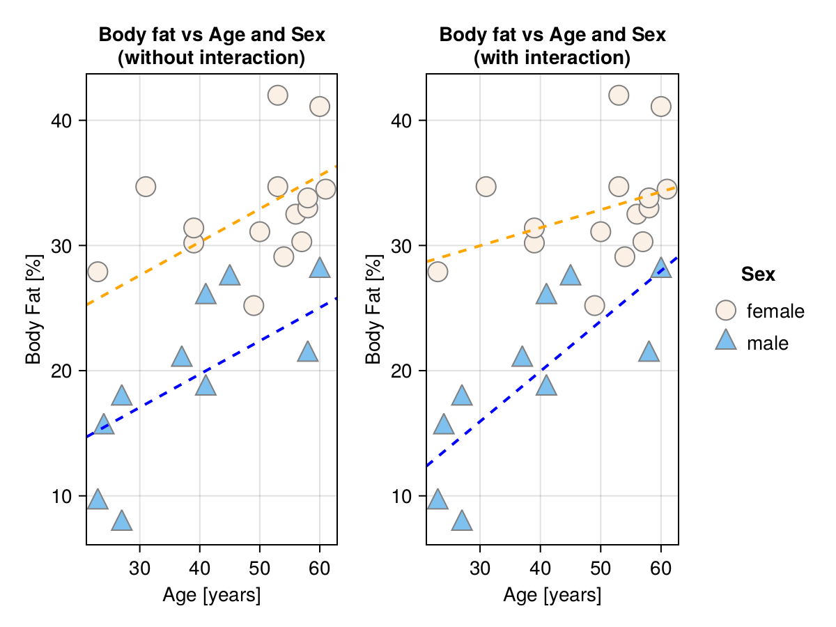
As you can see the model without interaction fits two regression lines (one for each Sex) with different intercepts, but the same slopes. On the other hand, the model with interaction fits two regression lines (one for each Sex) with different intercepts and different slopes. Since the coefficient (Coef.) for the interaction term (Age & Sex: male) is positive, this means that the slope for Sex: male is more steep (more positive). This would suggest that males tend to accumulate fat at a faster rate as they age.
So, when to use an interaction term in your model? The advice I heard was that in general, you should construct simple models and only use an interaction term when there are some good reasons for it. For instance, in the discussed case (agefat data frame), we might wanted to answer the research question: Does the accretion of body fat occurs faster in one of the genders as people age?