5.2 One sample Student’s t-test

Imagine that in your town there is a small local brewery that produces quite expensive but super tasty beer. You like it a lot, but you got an impression that the producer is not being honest with their customers and instead of the declared 500 [mL] of beer per bottle, he pours a bit less. Still, there is little you can do to prove it. Or can you?

You bought 10 bottles of beer (ouch, that was expensive!) and measured the volume of fluid in each of them. The results are as follows

# a representative sample
beerVolumes = [504, 477, 484, 476, 519, 481, 453, 485, 487, 501]

On a graph the volume distribution looks like this (it was drawn with Cmk.hist function).

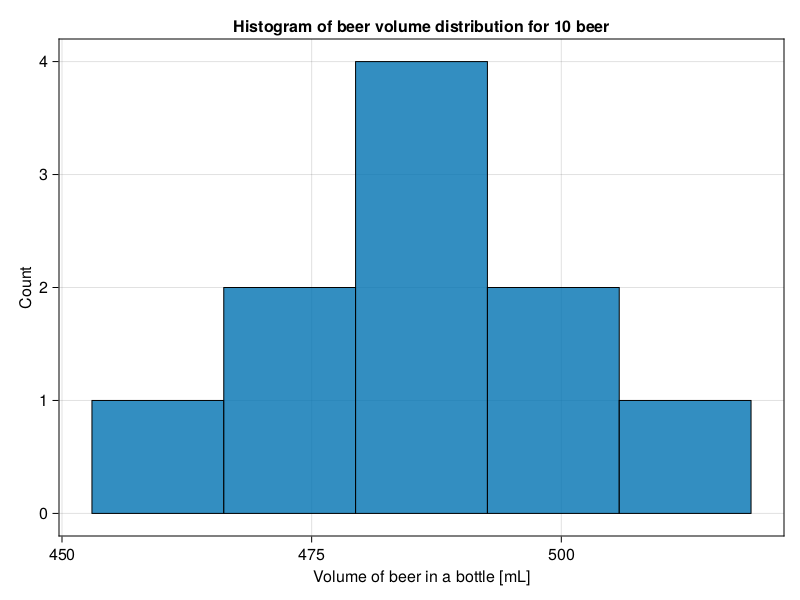
You look at it and it seems to resemble a bit the bell shaped curve that we discussed in the Section 4.6. This makes sense. Imagine your task is to pour let’s say 1’000 bottles daily with 500 [mL] of beer in each with a big mug (there is an erasable mark at a bottle’s neck). Most likely the volumes would oscillate around your goal volume of 500 [mL], but they would not be exact. Sometimes in a hurry you would add a bit more, sometimes a bit less (you could not waste time to correct it). So it seems like a reasonable assumption that the 1’000 bottles from our example would have a roughly bell shaped (aka normal) distribution of volumes around the mean.

Now you can calculate the mean and standard deviation for the data

import Statistics as Stats

meanBeerVol = Stats.mean(beerVolumes)
stdBeerVol = Stats.std(beerVolumes)

(meanBeerVol, stdBeerVol)

(486.7, 18.055777776410274)

Hmm, on average there was 486.7 [mL] of beer per bottle, but the spread of the data around the mean is also considerable (sd = 18.06 [mL]). The lowest value measured was 453 [mL], the highest value measured was 519 [mL]. Still, it seems that there is less beer per bottle than expected, but is it enough to draw a conclusion that the real mean in the population of our 1’000 bottles is ≈ 487.0 [mL] and not 500 [mL] as it should be? Let’s try to test that using what we already know about the normal distribution (see Section 4.6), the three sigma rule (Section 4.6.1) and the Distributions package (Section 4.6.2).

Let’s assume for a moment that the true mean for volume of fluid in the population of 1’000 beer bottles is meanBeerVol = 486.7 [mL] and the true standard deviation is stdBeerVol = 18.06 [mL]. That would be great because now, based on what we’ve learned in Section 4.6.2 we can calculate the probability that a random bottle of beer got >500 [mL] of fluid (or % of beer bottles in the population that contain >500 [mL] of fluid). Let’s do it

import Distributions as Dsts

# how many std. devs is value above or below the mean
function getZScore(value::Real, mean::Real, sd::Real)::Float64
    return (value - mean)/sd
end

expectedBeerVolmL = 500

fractionBeerLessEq500mL = Dsts.cdf(Dsts.Normal(),
    getZScore(expectedBeerVolmL, meanBeerVol, stdBeerVol))
fractionBeerAbove500mL = 1 - fractionBeerLessEq500mL

fractionBeerAbove500mL

0.2306808956300721

I’m not going to explain the code above since for reference you can always check Section 4.6.2. Still, under those assumptions roughly 0.23 or 23% of beer bottles contain more than 500 [mL] of fluid. In other words under these assumptions the probability that a random beer bottle contains >500 [mL] of fluid is 0.23 or 23%.

There are 2 problems with that solution.

Problem 1

It is true that the mean from the sample is our best estimate of the mean in the population (here 1’000 beer bottles poured daily). However, statisticians proved that instead of the standard deviation from our sample we should use the standard error of the mean. It describes the spread of sample means around the true population mean and it can be calculated as follows

\(sem = \frac{sd}{\sqrt{n}}\), where

sem - standard error of the mean

sd - standard deviation

n - number of observations in the sample

Let’s enclose it into Julia code

function getSem(vect::Vector{<:Real})::Float64
    return Stats.std(vect) / sqrt(length(vect))
end

Now we get a better estimate of the probability

fractionBeerLessEq500mL = Dsts.cdf(Dsts.Normal(),
    getZScore(expectedBeerVolmL, meanBeerVol, getSem(beerVolumes)))
fractionBeerAbove500mL = 1 - fractionBeerLessEq500mL

fractionBeerAbove500mL

0.00992016769999493

Under those assumptions the probability that a beer bottle contains >500 [mL] of fluid is roughly 0.01 or 1%.

So, to sum up. Here, we assumed that the true mean in the population is our sample mean (\(\mu\) = meanBeerVol). Next, if we were to take many small samples like beerVolumes and calculate their means then they would be normally distributed around the population mean (here \(\mu\) = meanBeerVol) with \(\sigma\) (standard deviation in the population) = getSem(beerVolumes). Finally, using the three sigma rule (see Section 4.6.1) we check if our hypothesized mean (expectedBeerVolmL) lies within roughly 2 standard deviations (here approximately 2 sems) from the assumed population mean (here \(\mu\) = meanBeerVol).

Problem 2

The sample size is small (length(beerVolumes) = 10) so the underlying distribution is quasi-normal (quasi - almost, as it were). It is called a t-distribution (for comparison of an exemplary normal and t-distribution see the figure below). Therefore to get a better estimate of the probability we should use a t-distribution.

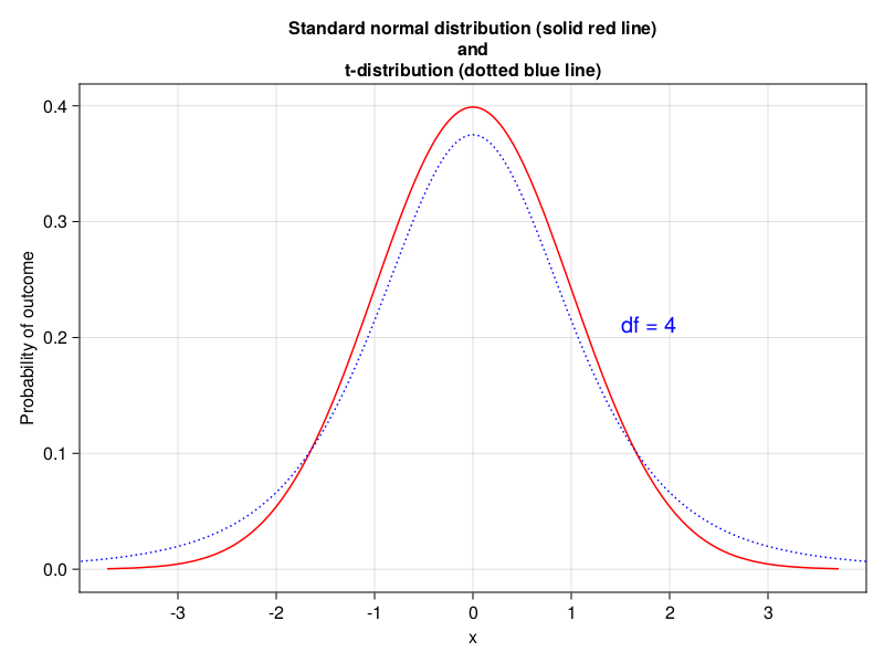
Luckily our Distributions package got the t-distribution included (see the docs). As you remember the normal distribution required two parameters that described it: the mean and the standard deviation. The t-distribution requires only the degrees of freedom. The concept is fairly easy to understand. Imagine that we recorded body masses of 3 people in the room: Paul, Peter, and John.

peopleBodyMassesKg = [84, 94, 78]

sum(peopleBodyMassesKg)

256

As you can see the sum of those body masses is 256 [kg]. Notice, however, that only two of those masses are independent or free to change. Once we know any two of the body masses (e.g. 94, 78) and the sum: 256, then the third body mass must be equal to sum(peopleBodyMassesKg) - 94 - 78 = 84 (it is determined, it cannot just freely take any value). So in order to calculate the degrees of freedom we type length(peopleBodyMassesKg) - 1 = 2. Since our sample size is equal to length(beerVolumes) = 10 then it will follow a t-distribution with length(beerVolumes) - 1 = 9 degrees of freedom.

So the probability that a beer bottle contains >500 [mL] of fluid is

function getDf(vect::Vector{<:Real})::Int
    return length(vect) - 1
end

fractionBeerLessEq500mL = Dsts.cdf(Dsts.TDist(getDf(beerVolumes)),
    getZScore(expectedBeerVolmL, meanBeerVol, getSem(beerVolumes)))
fractionBeerAbove500mL = 1 - fractionBeerLessEq500mL

fractionBeerAbove500mL

0.022397253591088795

Note: The z-score (number of standard deviations above or below the mean) for a t-distribution is called the t-score or t-statistics (it is calculated with sem instead of sd).

Finally, we got the result. Based on our representative sample (beerVolumes) and the assumptions we made we can see that the probability that a random beer contains >500 [mL] of fluid (500 [mL] is stated on a label) is fractionBeerAbove500mL = 0.022 or 2.2% (remember, this is one-tailed probability, the two-tailed probability is 0.022 * 2 = 0.044 = 4.4%).

Given that the cutoff level for \(\alpha\) (type I error) from Section 4.7.5 is 0.05 we can reject our \(H_{0}\) (the assumption that 500 [mL] comes from the population with the mean approximated by \(\mu\) = meanBeerVol = 486.7 [mL] and the standard deviation approximated by \(\sigma\) = sem = 5.71 [mL]).

In conclusion, our hunch was right (“…you got an impression that the producer is not being honest with their customers…”). The owner of the local brewery is dishonest and intentionally pours slightly less beer (on average expectedBeerVolmL - meanBeerVol = 13.0 [mL]). Now we can go to him and get our money back, or alarm the proper authorities for that monstrous crime. Fun fact: the story has it that the code of Hammurabi (circa 1750 BC) was the first to punish for diluting a beer with water (although it seems to be more of a legend). Still, this is like 2-3% beer (≈13/500 = 0.026) in a bottle less than it should be and the two-tailed probability (fractionBeerAbove500mL * 2 = 0.045) is not much less than the cutoff for type 1 error equal to 0.05 (we may want to collect a bigger sample and change the cutoff to 0.01).

5.2.1 HypothesisTests package

The above paragraphs were to further your understanding of the topic. In practice you can do this much faster using HypothesisTests package.

In our beer example you could go with this short snippet (see the docs for Htests.OneSampleTTest)

import HypothesisTests as Htests

Htests.OneSampleTTest(beerVolumes, expectedBeerVolmL)

One sample t-test
-----------------
Population details:
    parameter of interest:   Mean
    value under h_0:         500
    point estimate:          486.7
    95% confidence interval: (473.8, 499.6)

Test summary:
    outcome with 95% confidence: reject h_0
    two-sided p-value:           0.0448

Details:
    number of observations:   10
    t-statistic:              -2.329353706113303
    degrees of freedom:       9
    empirical standard error: 5.70973826993069

Let’s compare it with our previous results

(
expectedBeerVolmL, # value under h_0
meanBeerVol, # point estimate
fractionBeerAbove500mL * 2, # two-sided p-value
getZScore(expectedBeerVolmL, meanBeerVol, getSem(beerVolumes)),# t-statistic
getDf(beerVolumes), # degrees of freedom
getSem(beerVolumes) # empirical standard error
)

(500, 486.7, 0.04479450718217759, 2.329353706113303, 9, 5.70973826993069)

The numbers are pretty much the same (and they should be if the previous explanation was right). The t-statistic is positive in our case because getZScore subtracts mean from value (value - mean) and some packages (like HypothesisTests) swap the numbers.

The value that needs to be additionally explained is the 95% confidence interval from the output of HypothesisTests above. All it means is that: if we were to run our experiment with 10 beers 100 times and calculate 95% confidence intervals 100 times then 95 of the intervals would contain the true mean from the population. Sometimes people (over?)simplify it and say that this interval [in our case (473.8, 499.6)] contains the true mean from the population with probability of 95% (but that isn’t necessarily the same what was stated in the previous sentence). The narrower interval means better, more precise estimate. If the difference is statistically significant (p-value \(\le\) 0.05) then the interval should not contain the postulated mean (as it is in our case).

Notice that the obtained 95% confidence interval (473.8, 499.6) may indicate that the true average volume of fluid in a bottle of beer could be as high as 499.6 [mL] (so this would hardly make a practical difference) or as low as 473.8 [mL] (a small, ~6%, but a practical difference). In the case of our beer example it is just a curious fact, but imagine you are testing a new drug lowering the ‘bad cholesterol’ (LDL-C) level (the one that was mentioned in Section 4.9.5). Let’s say you got a 95% confidence interval for the reduction of (-132, +2). The interval encompasses 0, so the true effect may be 0 and you cannot reject \(H_{0}\) under those assumptions (p-value would be greater than 0.05). However, the interval is broad, and its lower value is -132, which means that the true reduction level after applying this drug could be even -132 [mg/dL]. Based on the data from this table I guess this could have a big therapeutic meaning. So, you might want to consider performing another experiment on the effects of the drug, but this time you should take a bigger sample to dispel the doubt (bigger sample size narrows the 95% confidence interval).

In general one sample t-test is used to check if a sample comes from a population with the postulated mean (in our case in \(H_{0}\) the postulated mean was 500 [mL]). However, I prefer to look at it from the different perspective (the other end) hence my explanation above. The t-test is named after William Sealy Gosset that published his papers under the pen-name Student, hence it is also called a Student’s t-test.

5.2.2 Checking the assumptions

Hopefully, the explanations above were clear enough. Still, we shouldn’t just jump into performing a test blindly, first we should test its assumptions (see figure below).

First of all we start by choosing a test to perform. Usually it is a parametric test, i.e. one that assumes some specific data distribution (e.g. normal). Then we check our assumptions. If they hold we proceed with our test. Otherwise we can either transform the data (e.g. take a logarithm from each value) or choose a different test (the one that got different assumptions or just less of them to fulfill). We will see an example of a data transformation, and the possible benefits it can bring us, later in this book (see the upcoming Section 7.8.1). Anyway, this different test usually belongs to so called non-parametric tests, i.e. tests that make less assumptions about the data, but are likely to be slightly less powerful (you remember the power of a test from Section 4.7.5, right?).

In our case a Student’s t-test requires (among others) the data to be normally distributed. This is usually verified with Shapiro-Wilk test or Kolmogorov-Smirnov test. As an alternative to Student’s t-test (when the normality assumption does not hold) a Wilcoxon test is often performed (of course before you use it you should check its assumptions, see Figure 14 above).

Both Kolmogorov-Smirnov (see this docs) and Wilcoxon test (see that docs) are at our disposal in HypothesisTests package. Behold

Htests.ExactOneSampleKSTest(beerVolumes,
    Dsts.Normal(meanBeerVol, stdBeerVol))

Exact one sample Kolmogorov-Smirnov test
----------------------------------------
Population details:
    parameter of interest:   Supremum of CDF differences
    value under h_0:         0.0
    point estimate:          0.193372

Test summary:
    outcome with 95% confidence: fail to reject h_0
    two-sided p-value:           0.7826

Details:
    number of observations:   10

So it seems we got no grounds to reject the \(H_{0}\) that states that our data are normally distributed (p-value > 0.05) and we were right to perform our one-sample Student’s t-test. Of course, I had checked the assumption before I conducted the test (Htests.OneSampleTTest). I didn’t mention it there because I didn’t want to prolong my explanation (and diverge from the topic) back there.

And now a question. Is the boring assumption check before a statistical test really necessary?

If you want your conclusions to reflect the reality well then yes. So, even though a statistical textbook for brevity may not check the assumptions of a method you should do it in your analyses if your care about the correctness of your judgment.