7.6 Simple Linear Regression

We began Section 7.2 with describing the relation between the volume of water and biomass of two plants of amazon rain forest. Let’s revisit the problem.

biomass
first(biomass, 5)

Effect of rainfall on plants biomass (fictitious data).

plantAkg	rainL	plantBkg
20.26	15.09	21.76
9.18	5.32	6.08
11.36	12.5	10.96
11.26	10.7	4.96
9.05	5.7	9.55

Previously, we said that the points are scattered around an imaginary line that goes through their center. Now, we could draw that line at a rough guess using a pen and a piece of paper (or a graphics editor). Based on the line we could make a prediction of the values on Y-axis based on the values on the X-axis. The variable placed on the X-axis is called independent (the rain does not depend on a plant, it falls or not), predictor or explanatory variable. The variable placed on the Y-axis is called dependent (the plant depends on rain) or outcome variable. The problem with drawing the line by hand is that it wouldn’t be reproducible, a line drawn by the same person would differ slightly from draw to draw. The same is true if a few different people have undertaken this task. Luckily, we got the simple linear regression, a method that allows us to draw the same line every single time based on a simple mathematical formula that takes the form:

\(y = a + b*x\), where:

• y - predicted value of y
• a - intercept (a point on Y-axis where the imaginary line crosses it at x = 0)
• b - slope (a value by which y increases/decreases when x changes by one unit)
• x - the value of x for which we want to estimate/predict the value of y

The slope (b) is fairly easy to calculate with Julia

function getSlope(xs::Vector{<:Real}, ys::Vector{<:Real})::Float64
    avgXs::Float64 = Stats.mean(xs)
    avgYs::Float64 = Stats.mean(ys)
    diffsXs::Vector{<:Real} = xs .- avgXs
    diffsYs::Vector{<:Real} = ys .- avgYs
    return sum(diffsXs .* diffsYs) / sum(diffsXs .^ 2)
end

getSlope (generic function with 1 method)

The function resembles the formula for the covariance that we met in Section 7.3. The difference is that there we divided sum(diffs1 .* diffs2) (here we called it sum(diffsXs .* diffsYs)) by the degrees of freedom (length(v1) - 1) and here we divide it by sum(diffsXs .^ 2). We might not have come up with the formula ourselves, still, it makes sense given that we are looking for the value by which y changes when x changes by one unit.

Once we got it, we may proceed to calculate the intercept (a) like so

function getIntercept(xs::Vector{<:Real}, ys::Vector{<:Real})::Float64
    return Stats.mean(ys) - getSlope(xs, ys) * Stats.mean(xs)
end

getIntercept (generic function with 1 method)

And now the results.

# be careful, unlike in getCor or getCov, here the order of variables
# in parameters influences the result
plantAIntercept = getIntercept(biomass.rainL, biomass.plantAkg)
plantASlope = getSlope(biomass.rainL, biomass.plantAkg)
plantBIntercept = getIntercept(biomass.rainL, biomass.plantBkg)
plantBSlope = getSlope(biomass.rainL, biomass.plantBkg)

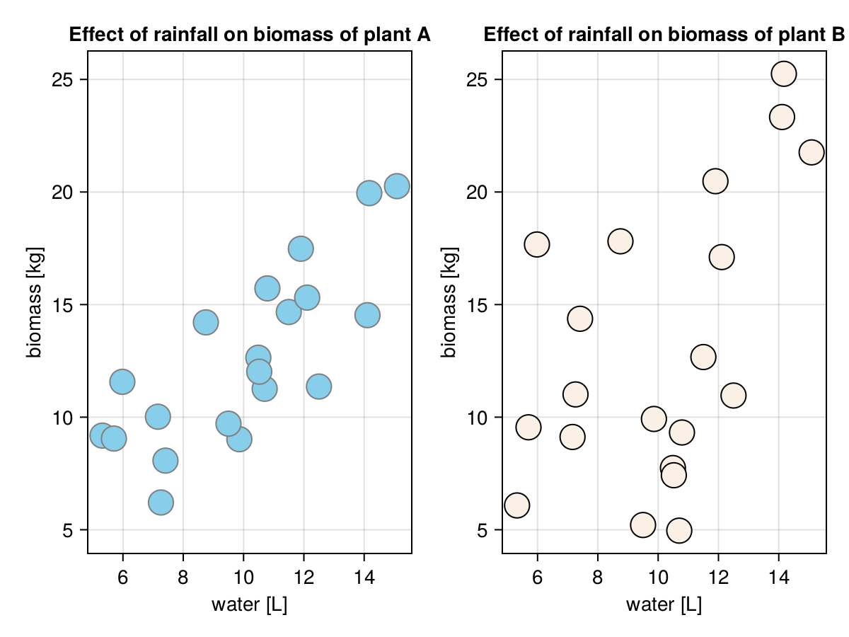
round.([plantASlope, plantBSlope], digits = 2)

[1.04, 1.14]

The intercepts are not our primary interest (we will explain why in a moment or two). We are more concerned with the slopes. Based on the slopes we can say that on average each additional liter or water (rainL) translates into 1.04 [kg] more biomass for plantA and 1.14 [kg] more biomass for plantB. Although, based on the correlation coefficients from Section 7.4 we know that the estimate for plantB is less precise. This is because the smaller correlation coefficient means a greater spread of the points along the line as can be seen in the figure below.

fig = Cmk.Figure()
ax1, sc1 = Cmk.scatter(fig[1, 1], biomass.rainL, biomass.plantAkg,
    markersize=25, color="skyblue", strokewidth=1, strokecolor="gray",
    axis=(; title="Effect of rainfall on biomass of plant A",
        xlabel="water [L]", ylabel="biomass [kg]")
)
ax2, sc2 = Cmk.scatter(fig[1, 2], biomass.rainL, biomass.plantBkg,
    markersize=25, color="linen", strokewidth=1, strokecolor="black",
    axis=(; title="Effect of rainfall on biomass of plant B",
        xlabel="water [L]", ylabel="biomass [kg]")
)
Cmk.ablines!(fig[1, 1],
    plantAIntercept,
    plantASlope,
    linestyle=:dash, color="gray")
Cmk.ablines!(fig[1, 2],
    plantBIntercept,
    plantBSlope,
    linestyle=:dash, color="gray")
Cmk.linkxaxes!(ax1, ax2)
Cmk.linkyaxes!(ax1, ax2)
fig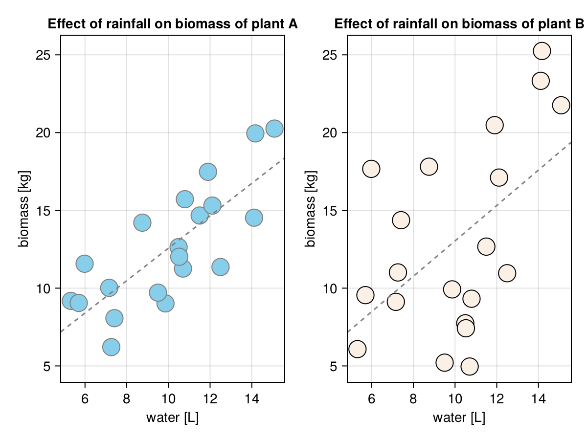

The trend line is placed more or less where we would have placed it at a rough guess, so it seems we got our functions right.

Now we can either use the graph (Figure 31) and read the expected value of the variable on the Y-axis based on a value on the X-axis (using a dashed line). Alternatively, we can write a formula based on \(y = a + b*x\) we mentioned before to get that estimate.

function getPrecictedY(
    x::Float64, intercept::Float64, slope::Float64)::Float64
    return intercept + slope * x
end

round.(
    getPrecictedY.([6.0, 10, 12], plantAIntercept, plantASlope),
    digits = 2)

[8.4, 12.57, 14.65]

It appears to work as expected (to confirm it read from Figure 31 values on Y-axis for the following values on X-axis: [6.0, 10, 12] using the dashed line for plantA).

OK, and now imagine you intend to introduce plantA into a botanic garden and you want it to grow well and fast. The function getPrecictedY tells us that if you pour 35 [L] of water to a field with plantA then on average you should get 42 [kg] of the biomass. Unfortunately after you applied the treatment it turned out the biomass actually dropped to 10 [kg] from the field. What happened? Reality. Most likely you (almost) drowned your plant. Lesson to be learned here. It is unsafe to use a model to make predictions beyond the data range on which it was trained. Ultimately, “All models are wrong, but some are useful”.

The above is the reason why in most cases we aren’t interested in the value of the intercept. The intercept is the value on the Y-axis when X is equal to 0, it is necessary for our model to work, but most likely it isn’t very informative (in our case a plant that receives no water simply dies).

So what is regression good for if it only enables us to make a prediction within the range on which it was trained? Well, if you ever underwent spirometry then you used regression in practice (or at least benefited from it). The functional examination of the respiratory system goes as follows. First, you enter your data: name, sex, height, weight, age, etc. Then you breathe (in a manner recommended by a technician) through a mouthpiece connected to an analyzer. Finally, you compare your results with the ones you should have obtained. If, let’s say your vital capacity is equal to 5.1 [L] and should be equal to 5 [L] then it is a good sign. However, if the obtained value is equal to 4 [L] when it should be 5 [L] (4/5 = 0.8 = 80% of the norm) then you should consult your physician. But where does the reference value come from?

One way to get it would be to rely on a large database, of let’s say 100-200 million healthy individuals (a data frame with 100-200 million rows and 5-6 columns for age, gender, height, etc. that is stored on a hard drive). Then all you have to do is to find a person (or people) whose data match yours exactly. Then you can take their vital capacity (or their a mean if there is more than one person that matches your features) as a reference point for yours. But this would be a great burden. For once you would have to collect data for a lot of individuals to be pretty sure that an exact combination of a given set of features occurs (hence the 100-200 million mentioned above). The other problem is that such a data frame would occupy a lot of disk space and would be slow to search through. A better solution is regression (most likely multiple linear regression that we will cover in Section 7.7). In that case you collect a smaller sample of let’s say 10’000 healthy individuals. You train your regression model. And store it together with the getPrecictedY function (where Y could be the discussed vital capacity). Now, you can easily and quickly calculate the reference value for a patient even if the exact set of features (values of predictor variables) was not in your training data set (still, you can be fairly sure that the values of the features of the patient are in the range of the training data set).

Anyway, in real life whenever you want to fit a regression line in Julia you should probably use GLM.jl package. In our case an exemplary output for plantA looks as follows.

import GLM as Glm

mod1 = Glm.lm(Glm.@formula(plantAkg ~ rainL), biomass)
mod1

plantAkg ~ 1 + rainL

Coefficients:
──────────────────────────────────────────────────────────────────────
               Coef.  Std. Error     t  Pr(>|t|)  Lower 95%  Upper 95%
──────────────────────────────────────────────────────────────────────
(Intercept)  2.14751    2.04177   1.05    0.3068  -2.14208     6.43711
rainL        1.04218    0.195771  5.32    <1e-04   0.630877    1.45347
──────────────────────────────────────────────────────────────────────

We begin with Glm.lm(formula, dataFrame) (lm stands for linear model). Next, we specify our relationship (Cmk.@formula) in the form Y ~ X, where Y is the dependent (outcome) variable, ~ is explained by, and X is the independent (explanatory) variable. This fits our model (mod1) to the data and yields quite some output.

The Coef. column contains the values of the intercept (previously estimated with getIntercept) and slope (before we used getSlope for that). It is followed by the Std. Error of the estimation (similar to the sem from Section 5.2). Then, just like in the case of the correlation (Section 7.4), some clever mathematical tweaking allows us to obtain a t-statistic for the Coef.s and p-values for them. The p-values tell us if the coefficients are really different from 0 (\(H_{0}\): a Coeff. is equal to 0) or estimate the probability that such a big value (or bigger) happened by chance alone (assuming that \(H_{0}\) is true). Finally, we end up with 95% confidence interval (similar to the one discussed in Section 5.2.1) that (oversimplifying stuff) tells us, with a degree of certainty, within what limits the true value of the coefficient in the population is.

We can use GLM to make our predictions as well.

round.(
    Glm.predict(mod1, Dfs.DataFrame(Dict("rainL" => [6, 10, 12]))),
    digits = 2
)

[8.4, 12.57, 14.65]

For that to work we feed Glm.predict with our model (mod1) and a DataFrame containing a column rainL that was used as a predictor in our model and voila, the results match those returned by getPrecictedY somewhat before in this section.

We can also get the general impression of how imprecise our prediction is by using the residuals (differences between the predicted and actual value on the Y-axis). Like so

# an average estimation error in prediction
# (based on abs differences)
function getAvgEstimError(
    lm::Glm.StatsModels.TableRegressionModel)::Float64
    return abs.(Glm.residuals(lm)) |> Stats.mean
end

getAvgEstimError(mod1)

2.075254994044967

So, on average our model miscalculates the value on the Y-axis (plantAkg) by 2 units (here kilograms). Of course, this is a slightly optimistic view, since we expect that on a new, previously unseen data set, the prediction error will be greater.

Moreover, the package allows us to calculate other useful stuff, like the coefficient of determination that tells us how much change in the variability on Y-axis is explained by our model (our explanatory variable(s)).

(
    Glm.r2(mod1),
    Stats.cor(biomass.rainL, biomass.plantAkg) ^ 2
)

(0.6115596392611107, 0.6115596392611111)

The coefficient of determination is called \(r^2\) (r squared) and in this case (simple linear regression) it is equal to the Pearson’s correlation coefficient (denoted as r) times itself. As we can see our model explains roughly 61% of variability in plantAkg biomass.