Probability distribution - Romeo and Julia, where Romeo is Basic Statistics

4.5 Probability distribution

Another important concept worth knowing is that of probability distribution. Let’s explore it with some, hopefully interesting, examples.

First, imagine I offer Your a bet. You roll two six-sided dice. If the sum of the dots is 12 then I give you $125, otherwise you give me $5. Hmm, sounds like a good bet, doesn’t it? Well, let’s find out. By flexing our probabilistic muscles and using a computer simulation this should not be too hard to answer.

function getSumOf2DiceRoll()::Int
    return sum(Rand.rand(1:6, 2))
end

Rand.seed!(321)
numOfRolls = 100_000
diceRolls = [getSumOf2DiceRoll() for _ in 1:numOfRolls]
diceCounts = getCounts(diceRolls)
diceProbs = getProbs(diceCounts)

Here, we rolled two 6-sided dice 100 thousand ($10^5$) times. The code introduces no new elements. The functions: getCounts, getProbs, Rand.seed! were already introduced in the previous chapter (see Section 4.4). And the for _ in construct we met while talking about for loops (see Section 3.6.1).

So, let’s take a closer look at the result.

(diceCounts[12], diceProbs[12])

(2780, 0.0278)

It seems that out of 100’000 rolls with two six-sided dice only 2780 gave us two sixes (6 + 6 = 12), so the experimental probability is equal to 0.0278. But is it worth it? From a point of view of a single person (remember the bet is you vs. me) a person got probability of diceProbs[12] = 0.0278 to win $125 and a probability of sum([get(diceProbs, i, 0) for i in 2:11]) = 0.9722 to lose $5. Since all the probabilities (for 2:12) add up to 1, the last part could be rewritten as 1 - diceProbs[12] = 0.9722. Using Julia I can write this in the form of an equation like so:

function getOutcomeOfBet(probWin::Float64, moneyWin::Real,
                         probLose::Float64, moneyLose::Real)::Float64
    # in mathematics first we do multiplication (*), then subtraction (-)
    return probWin * moneyWin - probLose * moneyLose
end

outcomeOf1bet = getOutcomeOfBet(diceProbs[12], 125, 1 - diceProbs[12], 5)

round(outcomeOf1bet, digits=2) # round to cents (1/100th of a dollar)

-1.39

In total you are expected to lose $ 1.39.

Now some people may say “Phi! What is $1.39 if I can potentially win $125 in a few tries”. It seems to me those are emotions (and perhaps greed) talking, but let’s test that too.

If 200 people make that bet (100 bet $5 on 12 and 100 bet $125 on the other result) we would expect the following outcome:

numOfBets = 100

outcomeOf100bets = (diceProbs[12] * numOfBets * 125) -
    ((1 - diceProbs[12]) * numOfBets * 5)
# or
outcomeOf100bets = ((diceProbs[12] * 125) - ((1 - diceProbs[12]) * 5)) * 100
# or simply
outcomeOf100bets = outcomeOf1bet * numOfBets

round(outcomeOf100bets, digits=2)

-138.6

OK. So, above we introduced a few similar ways to calculate that. The result of the bets is -138.6. In reality roughly 97 people that bet $5 on two sixes (6 + 6 = 12) lost their money and only 3 of them won $125 dollars which gives us $3*\$125 - 97*\$5= -\$110$ (the numbers are not exact because based on the probabilities we got, e.g. 2.78 people and not 3).

Interestingly, this is the same as if you placed that same bet with me 100 times. Ninety-seven times you would have lost $5 and only 3 times you would have won $125 dollars. This would leave you over $110 poorer and me over $110 richer ($110 transfer from you to me where the money should be).

It seems that instead of betting on 12 (two sixes) many times you would be better off had you started a casino or a lottery. Then you should find let’s say 1’000 people daily that will take that bet (or buy $5 ticket) and get you $ 1386.0 (outcomeOf1bet * 1000) richer every day (well, probably less, because you would have to pay some taxes, still this makes a pretty penny).

OK, you saw right through me and you don’t want to take that bet. Hmm, but what if I say a nice, big “I’m sorry” and offer you another bet. Again, you roll two six-sided dice. If you get 11 or 12 I give you $90 otherwise you give me $10. This time you know right away what to do:

pWin = sum([diceCounts[i] for i in 11:12]) / numOfRolls
# or
pWin = sum([diceProbs[i] for i in 11:12])

pLose = 1 - pWin

round(pWin * 90 - pLose * 10, digits=2)
# or
round(getOutcomeOfBet(pWin, 90, pLose, 10), digits=2)

-1.54

So, to estimate the probability we can either add number of occurrences of 11 and 12 and divide it by the total occurrences of all events OR, as we learned in the previous chapter (see Section 4.3), we can just add the probabilities of 11 and 12 to happen. Then we proceed with calculating the expected outcome of the bet and find out that I wanted to trick you again (“I’m sorry. Sorry.”).

Now, using this method (that relies on probability distribution) you will be able to look through any bet that I will offer you and choose only those that serve you well. OK, so what is a probability distribution anyway? Well, it is just the value that probability takes for any possible outcome. We can represent it graphically by using any of Julia’s plotting libraries.

Here, I’m going to use CairoMakie.jl which seems to produce pleasing to the eye plots and is simple enough (that’s what I think after I read its Basic Tutorial). Nota bene also its error messages are quite informative (once you learn to read them).

import CairoMakie as Cmk

function getSortedKeysVals(d::Dict{A,B})::Tuple{
    Vector{A},Vector{B}} where {A,B}

    sortedKeys::Vector{A} = keys(d) |> collect |> sort
    sortedVals::Vector{B} = [d[k] for k in sortedKeys]
    return (sortedKeys, sortedVals)
end

xs1, ys1 = getSortedKeysVals(diceCounts)
xs2, ys2 = getSortedKeysVals(diceProbs)

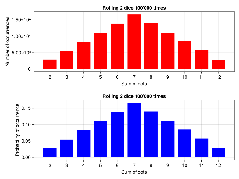
fig = Cmk.Figure()
Cmk.barplot(fig[1, 1:2], xs1, ys1,
    color="red",
    axis=(; # the ';' needs to be here
        title="Rolling 2 dice 100'000 times",
        xlabel="Sum of dots",
        ylabel="Number of occurrences",
        xticks=2:12)
)
Cmk.barplot(fig[2, 1:2], xs2, ys2,
    color="blue",
    axis=(; # the ';' needs to be here
        title="Rolling 2 dice 100'000 times",
        xlabel="Sum of dots",
        ylabel="Probability of occurrence",
        xticks=2:12)
)
fig

Note: Because of the compilation process running Julia’s plots for the first time may be slow. If that is the case you may try some tricks recommended by package designers, e.g. this one from the creators of Gadfly.jl.

First, we extracted the sorted keys and values from our dictionaries (diceCounts and diceProbs) using getSortedKeysVals. The only new element here is |> operator. It’s role is piping the output of one function as input to another function. So keys(d) |> collect |> sort is just another way of writing sort(collect(keys(d))). In both cases first we run keys(d), then we use the result of this function as an input to collect function, and finally pass its result to sort function. Out of the two options, the one with |> seems to be clearer to me.

Regarding the getSortedKeysVals it returns a tuple of sorted keys and values (that correspond with the sorted keys). In line xs1, ys1 = getSortedKeysVals(diceCounts) we unpack and assign them to xs1 (it gets the sorted keys) and ys1 (it gets values that correspond with the sorted keys). We do likewise for diceProbs in the line below.

In the next step we draw the distributions as bar plots (Cmk.barplot). The code seems to be pretty self explanatory after you read the tutorial that I just mentioned. Two points of notice here (in case you wanted to know more): 1) the axis=, color=, xlabel=, etc. are so called keyword arguments, 2) the axis keyword argument accepts a so called named tuple. OK, let’s get back to the graph. The number of counts (number of occurrences) on Y-axis is displayed using scientific notation, i.e. $1.0 x 10^4$ is 10’000 (one with 4 zeros) and $1.5 x 10^4$ is 15’000.

Figure 3: Rolling two 6-sided dice (counts and probabilities).

OK, but why did I even bother to talk about probability distributions (except for the great enlightenment it might have given to you)? Well, because it is important. It turns out that in statistics one relies on many probability distributions. For instance:

We want to know if people in city A are taller than in city B. We take at random 10 people from each of the cities, we measure them and run a famous Student’s T-test to find out. It gives us the probability that helps us answer our question. It does so based on a t-distribution (see the upcoming Section 5.3).
We want to know if cigarette smokers are more likely to believe in ghosts. What we do is we find random groups of smokers and non-smokers and ask them about it (Do you believe in ghosts?). We record the results and run a chi squared test that gives us the probability that helps us answer our question. It does so based on a chi squared distribution (see the upcoming Section 6.3).

OK, that should be enough for now. Take some rest, and when you’re ready continue to the next chapter.

4.4 Probability - theory and.. ← → 4.6 Normal distribution

CC BY-NC-SA 4.0 Bartlomiej Lukaszuk