7.3 Covariance

The formula for covariance resembles the one for variance that we met in Section 4.6 (getVar function) only that it is calculated for pairs of values (here a plant biomass and rainfall for a field), so two vectors instead of one. Observe

import Statistics as Stats

function getCov(v1::Vector{<:Real}, v2::Vector{<:Real})::Float64
    @assert length(v1) == length(v2) "v1 and v2 must be of equal lengths"
    avg1::Float64 = Stats.mean(v1)
    avg2::Float64 = Stats.mean(v2)
    diffs1::Vector{<:Real} = v1 .- avg1
    diffs2::Vector{<:Real} = v2 .- avg2
    return sum(diffs1 .* diffs2) / (length(v1) - 1)
end

Note: To calculate the covariance you may also use Statistics.cov.

A few points of notice. In Section 4.6 in getVar we squared the differences (diffs), i.e. we multiplied the diffs by themselves (\(x * x = x^2\)). Here, we do something similar by multiplying parallel values from both vectors of diffs (diffs1 and diffs2) by each other (\(x * y\), for a given field). Moreover, instead of taking the average (so sum(diffs1 .* diffs2)/length(v1)) here we use the more fine tuned statistical formula that relies on the degrees of freedom we met in Section 5.2 (there we used getDf function on a vector, here we kind of use getDf on the number of fields that are represented by the points in the Figure 27).

Enough explanations, let’s see how it works. First, a few possible associations that roughly take the following shapes on a graph: /, \, |, and -.

rowLenBiomass, _ = size(biomass)

(
    # assuming: getCov(xs, ys),
    # you may test the distributions with: Cmk.scatter(xs, ys)
    getCov(biomass.rainL, biomass.plantAkg), # /
    getCov(collect(1:1:rowLenBiomass), collect(rowLenBiomass:-1:1)), # \
    getCov(repeat([5], rowLenBiomass), biomass.plantAkg), # |
    getCov(biomass.rainL, repeat([5], rowLenBiomass)) # -
)

(8.721824210526316, -35.0, 0.0, 0.0)

We can see that whenever both variables (on X- and on Y-axis) increase simultaneously (points lie alongside / imaginary line like in Figure 27) then the covariance is positive. If one variable increases whereas the other decreases (points lie alongside \ imaginary line) then the covariance is negative. Whereas in the case when one variable changes and the other is stable (points lie alongside | or - line) the covariance is equal zero.

OK, time to compare the both plants.

covPlantA = getCov(biomass.plantAkg, biomass.rainL)
covPlantB = getCov(biomass.plantBkg, biomass.rainL)

(
    covPlantA,
    covPlantB,
)

(8.721824210526316, 9.527113684210526)

In Section 4.6 greater variance (and standard deviation) meant greater spread of points around the mean, here the greater covariance expresses the greater spread of the points around the imaginary trend line (in Figure 27). But beware, you shouldn’t judge the spread of data based on the covariance alone. To understand why let’s look at the graph below.

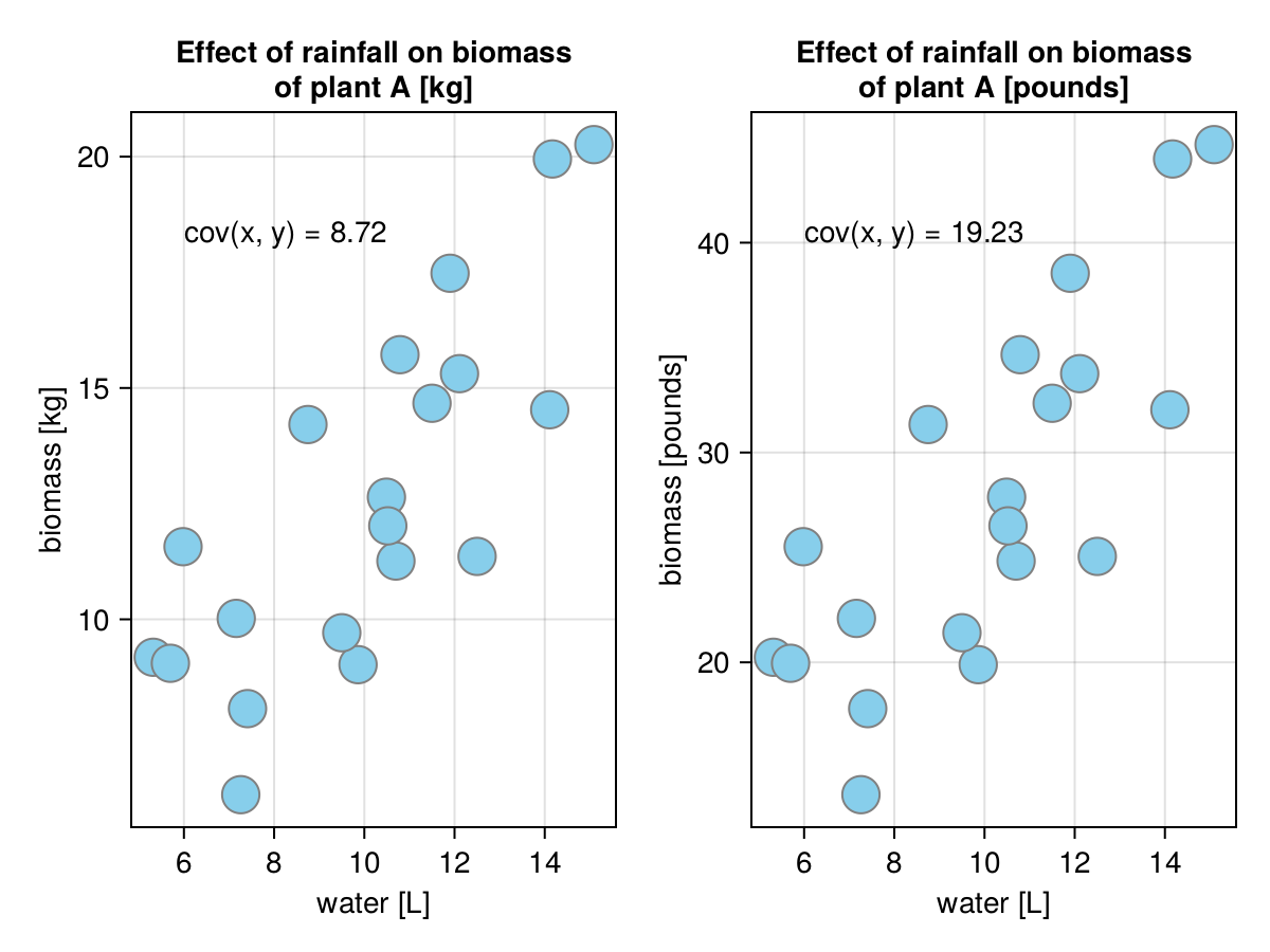
Here, we got the biomass of plantA in different units (kilograms and pounds). Logic and visual inspection of the points spread on the graph suggest that the covariances should be the same. Or maybe not?

(
    getCov(biomass.plantAkg, biomass.rainL),
    getCov(biomass.plantAkg .* 2.205, biomass.rainL),
)

(8.721824210526316, 19.231622384210525)

The covariances suggest that the spread of the data points is like 2 times greater between the two sub-graphs in Figure 28, but that is clearly not the case. The problem is that the covariance is easily inflated by the units of measurements. That is why we got an improved metrics for association named correlation.