4.7 Hypothesis testing
OK, now we are going to discuss a concept of hypothesis testing. But first let’s go through an example from everyday life that we know or at least can imagine. Ready?
4.7.1 A game of tennis
So imagine there is a group of people and among them two amateur tennis players: John and Peter. Everyone wants to know which one of them is a better tennis player. Well, there is only one way to find out. Let’s play some games!
As far as I’m aware a tennis match can end with a win of one player, the other loses (there are no draws). Before the games the people set the rules. Everyone agrees that the players will play six games. To prove their supremacy a player must win all six games (six wins in a row are unlikely to happen by accident, I hope we can all agree on that). The series of games ends with the result 0-6 for Peter. According to the previously set rules he is declared the local champion.
Believe it or not but this is what statisticians do. Of course they use more formal methodology and some mathematics, but still, this is what they do:
before the experiment they start with two assumptions
- initial assumption: be fair and assume that both players play equally well (this is called the null hypothesis, \(H_{0}\))
- alternative assumption: one player is better than the other (this is called the alternative hypothesis, \(H_{A}\))
before the experiment they decide on how big a sample should be (in our case six games).
before the experiment they decide on the cutoff level, once it is reached they will abandon the initial assumption (\(H_{0}\)) and chose the alternative (\(H_{A}\)). In our case the cutoff is: six games in a row won by a player
they conduct the experiment (players play six games) and record the results
after the experiment when the result provides enough evidence (in our case six games won by the same player) they decide to reject \(H_{0}\), and choose \(H_{A}\). Otherwise they stick to their initial assumption (they do not reject \(H_{0}\))
And that’s how it is, only that statisticians prefer to rely on probabilities instead of absolute numbers. So in our case a statistician says:
“I assume that \(H_{0}\) is true. Then I will conduct the experiment and record the result. I will calculate the probability of such a result (or a more extreme result) happening by chance. If it is small enough, let’s say 5% or less (\(prob \le 0.05\)), then the result is unlikely to have occurred by accident. Therefore I will reject my initial assumption (\(H_{0}\)) and choose the alternative (\(H_{A}\)). Otherwise I will stay with my initial assumption.”
Let’s see such a process in practice and connect it with what we already know.
4.7.2 Tennis - computer simulation
First a computer simulation.
# result of 6 tennis games under H0 (equally strong tennis players)
function getResultOf6TennisGames()
    return sum(Rand.rand(0:1, 6)) # 0 means John won, 1 means Peter won
end

Rand.seed!(321)
tennisGames = [getResultOf6TennisGames() for _ in 1:100_000]
tennisCounts = getCounts(tennisGames)
tennisProbs = getProbs(tennisCounts)
Here getResultOf6TennisGames returns a result of 6 games under \(H_0\) (both players got equal probability to win a game). When John wins a game then we get 0, when Peter we get 1. So if after running getResultOf6TennisGames we get, e.g. 4 we know that Peter won 4 games and John won 2 games. We repeat the experiment 100’000 times to get a reliable estimate of the results distribution.
OK, at the beginning of this chapter we intuitively said that a player needs to win 6 games to become the local champion. We know that the result was 0-6 for Peter. Let’s see what is the probability that Peter won by chance six games in a row (assuming \(H_{0}\) is true).
tennisProbs[6]0.01538
In this case the probability of Peter winning by chance six games in a row is very small. If we express it graphically it roughly looks like this:
# prob = 0.015
impossible ||||||||||||||||||||||||||||||||||||||||||||||||||| certain
            ∆
So, it seems that intuitively we set the cutoff level well. Let’s see if the statistician from the quotation above would be satisfied (“If it is small enough, let’s say 5% or less (\(prob \le 0.05\)), then the result is unlikely to have occurred by accident. Therefore I will reject my initial assumption (\(H_{0}\)) and choose the alternative (\(H_{A}\)). Otherwise I will stay with my initial assumption.”)
First, let’s compare them graphically.
# prob = 0.05
impossible ||||||||||||||||||||||||||||||||||||||||||||||||||| certain
             ∆

# prob = 0.0153
impossible ||||||||||||||||||||||||||||||||||||||||||||||||||| certain
            ∆
Although our text based graphics is slightly imprecise, we can see that the obtained probability lies below (to the left of) our cutoff level. And now more precise mathematical comparison.
# sigLevel - significance level for probability
# 5% = 5/100 = 0.05
function shouldRejectH0(prob::Float64, sigLevel::Float64 = 0.05)::Bool
    @assert (0 <= prob <= 1) "prob must be in range [0-1]"
    @assert (0 <= sigLevel <= 1) "sigLevel must be in range [0-1]"
    return prob <= sigLevel
end

shouldRejectH0(tennisProbs[6])
true
Indeed he would. He would have to reject \(H_{0}\) and assume that one of the players (here Peter) is a better player (\(H_{A}\)).
4.7.3 Tennis - theoretical calculations
OK, to be sure of our conclusions let’s try the same with the Distributions package (imported as Dsts) that we met before.
Remember one of the two tennis players must win a game (John or Peter). So this is a binomial distributions we met before. We assume (\(H_{0}\)) both of them play equally well, so the probability of any of them winning is 0.5. Now we can proceed like this using a dictionary comprehension similar to the one that we have met before (e.g. see getProbs definition from Section 4.4)
tennisTheorProbs = Dict(
    i => Dsts.pdf(Dsts.Binomial(6, 0.5), i) for i in 0:6
    )
tennisTheorProbs[6]
0.015624999999999977
Yep, the number is pretty close to tennisProbs[6] we got before which is 0.01538. So we decide to go with \(H_{A}\) and say that Peter is a better player. Just in case I will place both distributions (experimental and theoretical) one below the other to make the comparison easier. Behold
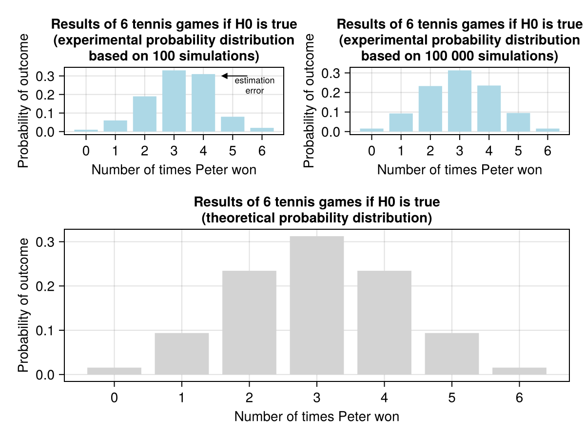
Notice that in order to get a satisfactory approximation of theoretical probabilities a sufficiently large number of repetitions needs to be ensured. Figure 8 (row 1, column 1) demonstrates an imprecise probability estimation obtained when only 100 computer simulations were used. In this case it could be noticed in few places, but it is especially evident in the case of overly large bar at x = 4 (indicated by the arrow).
Anyway, once we have warmed up we can even calculate the probability using our knowledge from Section 4.3.1. We can do this since by assuming our null hypothesis (\(H_{0}\)) we basically compared the result of a game between John and Peter to a fair coin’s toss (0 or 1, John or Peter, heads or tails).
The probability of Peter winning a single game is \(P(Peter) = \frac{1}{2} = 0.5\). Peter won all six games. In order to get two wins in a row, first he had to won one game. In order to get three wins in a row first he had to won two games in a row, and so on. So he had to win game 1 AND game 2 AND game 3 AND … . Given the above, and what we stated in Section 4.3.1, here we deal with a conjunction of probabilities. Therefore we use probability multiplication like so
tennisTheorProbWin6games = 0.5 * 0.5 * 0.5 * 0.5 * 0.5 * 0.5
# or
tennisTheorProbWin6games = 0.5 ^ 6

tennisTheorProbWin6games
0.015625
Compare it with tennisTheorProbs[6] calculated by Distributions package
(tennisTheorProbs[6], tennisTheorProbWin6games)(0.015624999999999977, 0.015625)They are the same. The difference is caused by a computer representation of floats and their rounding (as a reminder see Section 3.3.3, and Section 3.9.2).
Anyway, I just wanted to present all three methods for two reasons. First, that’s the way we checked our reasoning at math in primary school (solving with different methods). Second, chances are that one of the explanations may be too vague for you, if so help yourself to the other methods :)
In general, as a rule of thumb you should remember that the null hypothesis (\(H_{0}\)) assumes lack of differences/equality, etc. (and this is what we assumed in this tennis example).
4.7.4 One or two tails
Hopefully, the above explanations were clear enough. There is a small nuance to what we did. In the beginning of Section 4.7.1 we said ‘To prove their supremacy a player must win all six games’. A player, so either John or Peter. Still, we calculated only the probability of Peter winning the six games (tennisTheorProbs[6]), Peter and not John. What we did there was calculating one tail probability (see the figures in the link). Now, take a look at Figure 8 (e.g. bottom panel) the middle of it is ‘body’ and the edges to the left and right are tails.
This approach (one-tailed test) is rather OK in our case. However, in statistics it is frequently recommended to calculate two-tails probability (usually this is the default option in many statistical functions/packages). That is why at the beginning of Section 4.7.1 I wrote ‘alternative assumption: one player is better than the other (this is called alternative hypothesis, \(H_{A}\))’.
Calculating the two-tailed probability is very simple, we can either add tennisTheorProbs[6] + tennisTheorProbs[0] (remember 0 means that John won all six games) or multiply tennisTheorProbs[6] by 2 (since the graph in Figure 8 is symmetrical).
(tennisTheorProbs[6] + tennisTheorProbs[0], tennisTheorProbs[6] * 2)(0.031249999999999955, 0.031249999999999955)Once we got it we can perform our reasoning one more time.
shouldRejectH0(tennisTheorProbs[6] + tennisTheorProbs[0])true
In this case the decision is the same (but that is not always the case). As I said before in general it is recommended to choose a two-tailed test over a one-tailed test. Why? Let me try to explain this with another example.
Imagine I tell you that I’m a psychic that talks with the spirits and I know a lot of the stuff that is hidden from mere mortals (like the rank and suit of a covered playing card). You say you don’t believe me and propose a simple test.
You take 10 random cards from a deck. My task is to tell you the color (red or black). And I did, the only problem is that I was wrong every single time! If you think that proves that your were right in the first place then try to guess 10 cards in a row wrongly yourself (if you don’t have cards on you go with 10 consecutive fair coin tosses).
It turns out that guessing 10 cards wrong is just as unlikely as guessing 10 of them right (0.5^10 = 0.0009765625 or 1 per 1024 tries in each case). This could potentially mean a few things, e.g.
- I really talk with the spirits, but in their language “red” means “black”, and “black” means “red” (cultural fun fact: they say Bulgarians nod their heads when they say “no”, and shake them for “yes”),
- I live in one of 1024 alternative dimensions/realities and in this reality I managed to guess all of them wrong, when the other versions of me had mixed results, and that one version of me guessed all of them right,
- I am a superhero and have an x-ray vision in my eyes so I saw the cards, but I decided to tell them wrong to protect my secret identity,
- I cheated, and were able to see the cards beforehand, but decided to mock you,
- or some other explanation is in order, but I didn’t think of it right now.
The small probability only tells us that the result is unlikely to has happened by chance alone. Still, you should always choose your null (\(H_{0}\)) and alternative (\(H_{A}\)) hypothesis carefully. Moreover, it is a good idea to look at both ends of a probability distribution.
4.7.5 All the errors that we make
Long time ago when I was a student I visited a local chess club. I was late that day, and only one person was without a pair, Paul. I introduced myself and we played a few games. In chess you can either win, lose, or draw a game. Unfortunately, I lost all six games we played that day. I was upset, I assumed I just encountered a better player. I thought: “Too bad, but next week I will be on time and find someone else to play with” (nobody likes loosing all the time). The next week I came to the club, and again the only person without a pair was Paul (just my luck). Still, despite the bad feelings I won all six games that we played that day (what are the odds). Later on it turned out that me and Paul are pretty well matched chess players (we played chess at a similar level).
The story demonstrates that even when there is a lot of evidence (six lost games during the first meeting) we can still make an error by rejecting our null hypothesis (\(H_{0}\)).
In fact, whenever we do statistics we turn into judges, since we can make a mistake in two ways (see Figure 9).
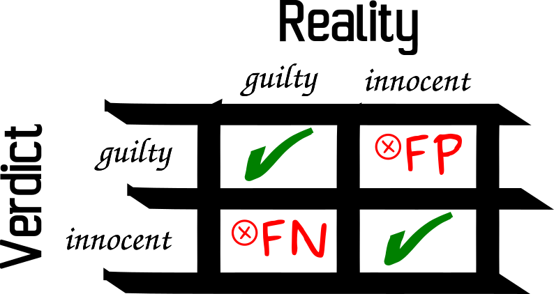
An accused is either guilty or innocent. A judge (or a jury in some countries) sets a verdict based on the evidence.
If the accused is innocent but is sentenced anyway then it is an error, it is usually called type I error (FP - false positive in Figure 9). Its probability is denoted by the first letter of the Greek alphabet, so alpha (α).
In the case of John and Peter playing tennis the type I probability was \(\le\) 0.05. More precisely it was tennisTheorProbs[6] = 0.015625 (for a one tailed test).
If the accused is guilty but is declared innocent then it is another type of error, it is usually called type II error (FN - false negative in Figure 9). Its probability is denoted by the second letter of the Greek alphabet, so beta (β). Beta helps us determine the power of a test (power = 1 - β), i.e. if \(H_{A}\) is really true then how likely it is that we will choose \(H_{A}\) over \(H_{0}\).
So to sum up, in the judge analogy a really innocent person is \(H_{0}\) being true and a really guilty person is \(H_{A}\) being true.
Unfortunately, most of the statistical textbooks that I’ve read revolve around type I errors and alphas, whereas type II error is covered much less extensively (hence my own knowledge of the topic is more limited).
In the tennis example above we rejected \(H_{0}\), hence here we risk committing the type I error. Therefore, we didn’t speak about the type II error, but don’t worry we will discuss it in more detail in the upcoming exercises at the end of this chapter (see Section 4.8.5).
4.7.6 Cutoff levels
OK, once we know what are the type I and type II errors it is time to discuss their cutoff values.
Obviously, the ideal situation would be if the probabilities of both type I and type II errors were exactly 0 (no mistakes is always the best). The only problem is that this is not possible. In our tennis example one player won all six games, and still some small risk of a mistake existed (tennisTheorProbs[6] = 0.015625). If you ever see a statistical package reporting a p-value to be equal, e.g. 0.0000, then this is just rounding to 4 decimal places and not an actual zero. So what are the acceptable cutoff levels for \(\alpha\) (probability of type I error) and \(\beta\) (probability of type II error).
The most popular choices for \(\alpha\) cutoff values are:
- 0.05, or
- 0.01
Actually, as far as I’m aware, the first of them (\(\alpha = 0.05\)) was initially proposed by Ronald Fisher, a person sometimes named the father of the XX-century statistics. This value was chosen arbitrarily and is currently frowned upon by some modern statisticians as being to lenient. Therefore, 0.01 is proposed as a more reasonable alternative.
As regards \(\beta\) its two most commonly accepted cutoff values are:
- 0.2, or
- 0.1
Actually, as far as I remember the textbooks usually do not report values for \(\beta\), but for power of the test (if \(H_{A}\) is really true then how likely it is that we will choose \(H_{A}\) over \(H_{0}\)) to be 0.8 or 0.9. However, since as we mentioned earlier power = 1 - \(\beta\), then we can easily calculate the value for this parameter.
OK, enough of theory, time for some practice. Whenever you’re ready click the right arrow to proceed to the exercises that I prepared for you.