6.8 Solutions - Comparisons of Categorical Data
In this sub-chapter you will find exemplary solutions to the exercises from the previous section.
6.8.1 Solution to Exercise 1
An exemplary getContingencyTable could look like this (here, a version that produces output that resembles the result of FreqTables.freqtable):
function getContingencyTable(
    rowVect::Vector{String},
    colVect::Vector{String},
    rowLabel::String,
    colLabel::String,
    )::Dfs.DataFrame

    rowNames::Vector{String} = sort(unique(rowVect))
    colNames::Vector{String} = sort(unique(colVect))
    pairs::Vector{Tuple{String, String}} = collect(zip(rowVect, colVect))
    pairsCounts::Dict{Tuple{String, String}, Int} = getCounts(pairs)
    labels::String = "↓" * rowLabel * "/" * colLabel * "→"
    df::Dfs.DataFrame = Dfs.DataFrame()
    columns::Dict{String, Vector{Int}} = Dict()

    for cn in colNames
        columns[cn] = [get(pairsCounts, (rn, cn), 0) for rn in rowNames]
    end

    df = Dfs.DataFrame(columns)
    Dfs.insertcols!(df, 1, labels => rowNames)

    return df
end
Here, as we often do, we start by declaring some of the helpful variables. rowNames and colNames contain all the possible unique groups for each input variable (rowVect and colVect). Then we get all the consecutive pairings that are in the data by using zip and collect functions. For instance collect(zip(["a", "a", "b"], ["x", "y", "x"])) will yield us the following vector of tuples: [("a", "x"), ("a", "y"), ("b", "x")]. The pairs are then sent to getCounts (from Section 4.4) to find out how often a given pair occurs.
In the next step we define a variable df (for now it is empty) to hold our final result. We saw in Section 6.3 that a data frame can be created by sending a dictionary to the Dfs.DataFrame function. Therefore, we declare columns (a dictionary) that will hold the count for every column of our contingency table.
We fill the columns one by one with for cn in colNames loop. To get a count for a particular row of a given column ((rn, cn)) we use get function that extracts it from pairsCounts. If the key is not there (a given combination of (rn, cn) does not exist) we return 0 as a default value. We fill columns by using comprehensions (see Section 3.6.3).
Finally, we put our counts (columns) into the data frame (df). Now, we insert a column with rowNames at position 1 (first column from left) with Dfs.insertcols!.
All that it is left to do is to return the result.
Let’s find out how our getContingencyTable works.
smokersByProfession = getContingencyTable(
    smoker,
    profession,
    "smoker",
    "profession"
)
| ↓smoker/profession→ | Lawyer | Priest | Teacher |
|---|---|---|---|
| no | 14 | 11 | 18 |
| yes | 17 | 20 | 20 |
It appears to work just fine. Let’s swap the inputs and see if we get a consistent result.
smokersByProfessionTransposed = getContingencyTable(
    profession,
    smoker,
    "profession",
    "smoker"
)
| ↓profession/smoker→ | no | yes |
|---|---|---|
| Lawyer | 14 | 17 |
| Priest | 11 | 20 |
| Teacher | 18 | 20 |
Looks good. And now for the small data set with possible zeros.
smokersByProfessionSmall = getContingencyTable(
    smokerSmall,
    professionSmall,
    "smoker",
    "profession"
)
| ↓smoker/profession→ | Lawyer | Priest | Teacher |
|---|---|---|---|
| no | 2 | 3 | 1 |
| yes | 0 | 1 | 3 |
Seems to be OK as well. Of course we can use this function with a data frame, e.g. getContingencyTable(df[!, "col1"], df[!, "col2"], "col1", "col2") or adopt it slightly to take a data frame as an input.
6.8.2 Solution to Exercise 2
OK, the most direct solution to the problem (for getColPerc) would be something like
function getColPerc(m::Matrix{Int})::Matrix{Float64}
    nRows, nCols = size(m)
    percentages:: Matrix{Float64} = zeros(nRows, nCols)
    for c in 1:nCols
        for r in 1:nRows
            percentages[r, c] = m[r, c] / sum(m[:, c])
            percentages[r, c] = round(percentages[r, c] * 100, digits = 2)
        end
    end
    return percentages
end
Here, we begin by extracting the number of rows (nRows) and columns (nCols). We use them right away by defining percentages matrix that will hold our final result (for now it is filled with 0s). Then we use the classical nested for loops idiom to calculate the percentage for every cell in the matrix/table (we use array indexing we met in Section 3.3.7). For that we divide each count (m[r, c]) by column sum (sum(m[:, c])). Next, we multiply it by 100 (* 100) to change the decimal to percentage. We round the percentage to two decimal points (round and digits = 2).
The algorithm is not super efficient (we calculate sum(m[:, c]) separately for every cell) or terse (9 lines of code). Still, it is pretty clear and for small matrices (a few/several rows/cols, that we expect in our input) does the trick.
OK, let’s move to the getRowPerc function.
function getRowPerc(m::Matrix{Int})::Matrix{Float64}
    nRows, nCols = size(m)
    percentages:: Matrix{Float64} = zeros(nRows, nCols)
    for c in 1:nCols
        for r in 1:nRows
            percentages[r, c] = m[r, c] / sum(m[r, :])
            percentages[r, c] = round(percentages[r, c] * 100, digits = 2)
        end
    end
    return percentages
end
Hmm, it’s almost identical to getColPerc (sum(m[:, c]) was replaced with sum(m[r, :])). Let’s remove the code duplication and put it into a single function.
function getPerc(m::Matrix{Int}, byRow::Bool)::Matrix{Float64}
    nRows, nCols = size(m)
    percentages:: Matrix{Float64} = zeros(nRows, nCols)
    dimSum::Int = 0 # sum in a given dimension of a matrix
    for c in 1:nCols
        for r in 1:nRows
            dimSum = (byRow ? sum(m[r, :]) : sum(m[:, c]))
            percentages[r, c] = m[r, c] / dimSum
            percentages[r, c] = round(percentages[r, c] * 100, digits = 2)
        end
    end
    return percentages
end
Here, we replaced the function specific sums with a more general dimSum (initialized with 0). Then inside the inner for loop we decide which sum to compute (row sum with sum(m[r, :]) and column sum with sum(m[:, c])) with a ternary expression from Section 3.5.2. OK, enough of tweaking and code optimization, let’s test our new function.
mEyeColor2×2 Matrix{Int64}:
220 161
279 320And now column percentages
eyeColorColPerc = getPerc(mEyeColor, false)
eyeColorColPerc
2×2 Matrix{Float64}:
44.09 33.47
55.91 66.53So, based on the data in mEyeColor we see that in the uk (first column) there is roughly 44.09% of people with blue eyes. Whereas in the us (second column) there is roughly 33.47% of people with that eye color.
And now for the row percentages.
eyeColorRowPerc = getPerc(mEyeColor, true)
eyeColorRowPerc
2×2 Matrix{Float64}:
57.74 42.26
46.58 53.42So, based on the data in mEyeColor we see that among the investigated groups roughly 57.74% of blue eyed people live in the uk and 42.26% of blue eyed people live in the us.
OK, let’s just quickly make sure our function also works fine for a bigger table.
mEyeColorFull3×2 Matrix{Int64}:
220 161
149 78
130 242And now column percentages.
eyeColorColPercFull = getPerc(mEyeColorFull, false)
eyeColorColPercFull
3×2 Matrix{Float64}:
44.09 33.47
29.86 16.22
26.05 50.31So, based on the data in mEyeColor we see that in the uk (first column) there is roughly:
- 44.09% of people with blue eyes,
- 29.86% of people with green eyes, and
- 26.05% of people with brown eyes.
For us (second column) we got:
- 33.47% of people with blue eyes,
- 16.22% of people with green eyes, and
- 50.31% of people with brown eyes.
Of course, remember that this is all fictitious data inspired by the lecture of this Wikipedia’s page.
OK, enough for the task solution. If you want to see a more terse (and mysterious) version of getPerc then go to this chapter’s code snippets.
6.8.3 Solution to Exercise 3
OK, the most straightforward way to draw a stacked bar plot would be to use Cmk.barplot with stack and color keyword arguments.
The solution below is slightly different. It allows for greater control over the output and it was created after some try and error.
import CairoMakie as Cmk

function drawColPerc(df::Dfs.DataFrame,
    dfColLabel::String,
    dfRowLabel::String,
    title::String,
    dfRowColors::Vector{String})::Cmk.Figure

    m::Matrix{Int} = Matrix{Int}(df[:, 2:end])
    columnPerc::Matrix{Float64} = getPerc(m, false)
    nRows, nCols = size(columnPerc)
    colNames::Vector{String} = names(df)[2:end]
    rowNames::Vector{String} = df[1:end, 1]
    xs::Vector{Int} = collect(1:nCols)
    offsets::Vector{Float64} = zeros(nCols)
    curPerc::Vector{Float64} = []
    barplots = []

    fig = Cmk.Figure()
    ax1 = Cmk.Axis(fig[1, 1],
                   title=title, xlabel=dfColLabel, ylabel="% of data",
                   xticks=(xs, colNames), yticks=0:10:100)

    for r in 1:nRows
        curPerc = columnPerc[r, :]
        push!(barplots,
            Cmk.barplot!(ax1, xs, curPerc,
                         offset=offsets, color=dfRowColors[r]))
        offsets = offsets .+ curPerc
    end
    Cmk.Legend(fig[1, 2], barplots, rowNames, dfRowLabel)

    return fig
end
We begin by defining a few helpful variables. Most of them are pretty self explanatory and rely on the constructs we met before. The three most enigmatic are offsets, curPerc, and barplots.
offsets are the locations on Y-axis where the bottom edges of the bars will be drawn (it is initialized with zeros). curPerc will contain heights of the bars to be drawn. barplots will contain a vector of bar plot objects drawn (it is necessary for adding proper legend with Cmk.Legend). For each row in columnPerc (for r in 1:nRows) we take the percentage of the row and put it into curPerc. Then we draw bars (Cmk.barplot!) of that height that start (their bottom edges) at offsets and are of a color of our choosing (dfRowColors[r]). The list of allowed named colors can be found here. We append the drawn bars to the bars vector by using push! function (we met it in Section 3.4.4). Then we add curPerc to the offset so that the bottom edges of the next bars will start where the top edges of the previous bars ended.
Once the for loop ended we finish by adding the appropriate legend.
OK, time to test our function
drawColPerc(dfEyeColorFull, "Country", "Eye color",
    "Eye Color distribution by country (column percentages)",
    ["lightblue1", "seagreen3", "peachpuff3"])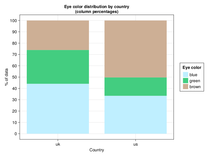
I don’t know about you but to me it looks pretty nice.
OK, now we could write drawRowPerc function by modifying our drawColPerc slightly. Finally, after some try and error we could write drawPerc function that combines both those functionalities and reduces code duplication. Without further ado let me fast forward to the definition of drawPerc
function drawPerc(df::Dfs.DataFrame, byRow::Bool,
    dfColLabel::String,
    dfRowLabel::String,
    title::String,
    groupColors::Vector{String})::Cmk.Figure

    m::Matrix{Int} = Matrix{Int}(df[:, 2:end])
    dimPerc::Matrix{Float64} = getPerc(m, byRow)
    nRows, nCols = size(dimPerc)
    colNames::Vector{String} = names(df)[2:end]
    rowNames::Vector{String} = df[1:end, 1]
    ylabel::String = "% of data"
    xlabel::String = (byRow ? dfRowLabel : dfColLabel)
    xs::Vector{Int} = collect(1:nCols)
    yticks::Tuple{Vector{Int},Vector{String}} = (
        collect(0:10:100), map(string, 0:10:100)
    )
    xticks::Tuple{Vector{Int},Vector{String}} = (xs, colNames)

    if byRow
        nRows, nCols = nCols, nRows
        xs = collect(1:nCols)
        colNames, rowNames = rowNames, colNames
        dfColLabel, dfRowLabel = dfRowLabel, dfColLabel
        xlabel, ylabel = ylabel, xlabel
        yticks, xticks = (xs, colNames), yticks
    end

    offsets::Vector{Float64} = zeros(nCols)
    curPerc::Vector{Float64} = []
    barplots = []

    fig = Cmk.Figure()
    ax1 = Cmk.Axis(fig[1, 1], title=title,
                   xlabel=xlabel, ylabel=ylabel,
                   xticks=xticks, yticks=yticks)

    for r in 1:nRows
        curPerc = (byRow ? dimPerc[:, r] : dimPerc[r, :])
        push!(barplots,
            Cmk.barplot!(ax1, xs, curPerc,
                         offset=offsets, color=groupColors[r],
                         direction=(byRow ? :x : :y)))
        offsets = offsets .+ curPerc
    end
    Cmk.Legend(fig[1, 2], barplots, rowNames, dfRowLabel)

    return fig
end
Ok, let’s see how it works.
drawPerc(dfEyeColorFull, true,
    "Country", "Eye color",
    "Eye Color distribution by country (row percentages)",
    ["red", "blue"])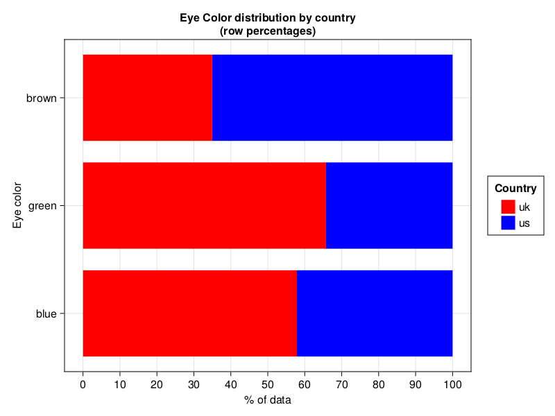
Pretty, pretty, pretty.
I leave the code in drawPerc for you to decipher. Let me just explain a few new pieces.
In Julia (like in Python) we can define two variables in one go by using the following syntax: a, b = 1, 2 (now a = 1 and b = 2). Let’s say that later in our program we decided that from now on a should be 2, and b should be 1. We can swap the variables using the following one line expression: a, b = b, a.
Additionally, drawPerc makes use of the direction keyword argument that accepts symbols :x or :y. It made the output slightly more visually pleasing but also marginally complicated the code. Anyway, direction = :y draws vertical bars (see Figure 24), whereas direction = :x draws horizontal bars (see Figure 25).
And that’s it for this exercise.
6.8.4 Solution to Exercise 4
OK, let’s start by defining helper functions that we will use to test the assumptions.
function isSumAboveCutoff(m::Matrix{Int}, cutoff::Int = 49)::Bool
    return sum(m) > cutoff
end

function getExpectedCounts(m::Matrix{Int})::Vector{Float64}
    nObs::Int = sum(m)
    cProbs::Vector{Float64} = [sum(c) / nObs for c in eachcol(m)]
    rProbs::Vector{Float64} = [sum(r) / nObs for r in eachrow(m)]
    probsUnderH0::Vector{Float64} = [
        cp * rp for cp in cProbs for rp in rProbs
        ]
    return probsUnderH0 .* nObs
end

function areAllExpectedCountsAboveCutoff(
    m::Matrix{Int}, cutoff::Float64 = 5.0)::Bool
    expectedCounts::Vector{Float64} = getExpectedCounts(m)
    return map(x -> x >= cutoff, expectedCounts) |> all
end

function areChiSq2AssumptionsOK(m::Matrix{Int})::Bool
    sumGTEQ50::Bool = isSumAboveCutoff(m)
    allExpValsGTEQ5::Bool = areAllExpectedCountsAboveCutoff(m)
    return sumGTEQ50 && allExpValsGTEQ5
end
There is not much to explain here, since all we did was to gather the functionality we had developed in the previous chapters (e.g. in Section 6.3).
And now for the tests.
function runFisherExactTestGetPVal(m::Matrix{Int})::Float64
    @assert (size(m) == (2, 2)) "input matrix must be of size (2, 2)"
    a, c, b, d = m
    return Ht.FisherExactTest(a, b, c, d) |> Ht.pvalue
end

function runCategTestGetPVal(m::Matrix{Int})::Float64
    @assert (size(m) == (2, 2)) "input matrix must be of size (2, 2)"
    if areChiSq2AssumptionsOK(m)
        return Ht.ChisqTest(m) |> Ht.pvalue
    else
        return runFisherExactTestGetPVal(m)
    end
end

function runCategTestGetPVal(df::Dfs.DataFrame)::Float64
    @assert (size(df) == (2, 3)) "input df must be of size (2, 3)"
    return runCategTestGetPVal(Matrix{Int}(df[:, 2:3]))
end
Again, all we did here was to collect the proper functionality we had developed in this chapter (Section 6) and its sub-chapters. Therefore, I’ll refrain myself from comments. Instead let’s test our newly developed tools.
round.(
    [
        runCategTestGetPVal(mEyeColor),
        runCategTestGetPVal(mEyeColorSmall),
        runCategTestGetPVal(dfEyeColor)
    ],
    digits = 4
)
[0.0007, 0.6373, 0.0007]The functions appear to be working as intended, and the obtained p-values match those from Section 6.3 and Section 6.4.
6.8.5 Solution to Exercise 5
Let’s start by writing a function that will accept a data frame like dfEyeColorFull and return all the possible 2x2 data frames (2 rows and 2 columns with counts).
# previously (ch05) defined function
function getUniquePairs(names::Vector{T})::Vector{Tuple{T,T}} where T
    @assert (length(names) >= 2) "the input must be of length >= 2"
    uniquePairs::Vector{Tuple{T,T}} =
        Vector{Tuple{T,T}}(undef, binomial(length(names), 2))
    currInd::Int = 1
    for i in eachindex(names)[1:(end-1)]
        for j in eachindex(names)[(i+1):end]
            uniquePairs[currInd] = (names[i], names[j])
            currInd += 1
        end
    end
    return uniquePairs
end

function get2x2Dfs(biggerDf::Dfs.DataFrame)::Vector{Dfs.DataFrame}
    nRows, nCols = size(biggerDf)
    @assert ((nRows > 2) || (nCols > 3)) "matrix of counts must be > 2x2"
    rPairs::Vector{Tuple{Int, Int}} = getUniquePairs(collect(1:nRows))
    # counts start from column 2
    cPairs::Vector{Tuple{Int, Int}} = getUniquePairs(collect(2:nCols))
    return [
        biggerDf[[r...], [1, c...]] for r in rPairs for c in cPairs
    ]
end
We begin by copying and pasting getUniquePairs from Section 5.8.4. We will use it in get2x2Dfs. First we get unique pairs of rows (rPairs). Then we get unique pairs of columns (cPairs). Finally, using nested comprehension and indexing (for reminder see Section 3.3.7 and Section 5.3.1) we get the vector of all possible 2x2 data frames (actually 2x3 data frames, because first column contains row labels). Since each element of rPairs (r) or cPairs (c) is a tuple, and indexing must be a vector, then we convert one into the other using [r...] and [c...] syntax (e.g. [(1, 2)...] will give us [1, 2]). In the end we get the list of data frames as a result.
OK, let’s write a function to compute p-values (for now unadjusted) for data frames in a vector.
function runCategTestsGetPVals(
    biggerDf::Dfs.DataFrame
    )::Tuple{Vector{Dfs.DataFrame}, Vector{Float64}}

    overallPVal::Float64 = Ht.ChisqTest(
        Matrix{Int}(biggerDf[:, 2:end])) |> Ht.pvalue
    if (overallPVal <= 0.05)
        dfs::Vector{Dfs.DataFrame} = get2x2Dfs(biggerDf)
        pvals::Vector{Float64} = runCategTestGetPVal.(dfs)
        return (dfs, pvals)
    else
        return ([biggerDf], [overallPVal])
    end
end
The function is rather simple. First, it checks the overall p-value (overallPVal) for the biggerDf. If it is less than or equal to our customary cutoff level (\(\alpha = 0.05\)) then we execute runCategTestGetPVal on each possible data frame (dfs) using the dot operator syntax from Section 3.6.5. We return a tuple, its first element is a vector of data frames, its second element is a vector of corresponding (uncorrected) p-values. If overallPVal is greater than the cutoff level then we place our biggerDf and its corresponding p-value (overallPVal) into vectors, and place them into a tuple (which is returned).
Time to test our function.
resultCategTests = runCategTestsGetPVals(dfEyeColorFull)
resultCategTests[1]| eyeCol | uk | us |
|---|---|---|
| blue | 220 | 161 |
| green | 149 | 78 |
| eyeCol | uk | us |
|---|---|---|
| blue | 220 | 161 |
| brown | 130 | 242 |
| eyeCol | uk | us |
|---|---|---|
| green | 149 | 78 |
| brown | 130 | 242 |
Looking good, and now the corresponding unadjusted p-values.
resultCategTests[2][0.05384721765961758, 3.5949791158435336e-10, 2.761179458504292e-13]Once we got it, adjusting the p-values should be a breeze.
import MultipleTesting as Mt

function adjustPVals(
    multCategTestsResults::Tuple{Vector{Dfs.DataFrame}, Vector{Float64}},
    multCorr::Type{<:Mt.PValueAdjustment}
    )::Tuple{Vector{Dfs.DataFrame}, Vector{Float64}}
    dfs, pvals = multCategTestsResults
    adjPVals::Vector{Float64} = Mt.adjust(pvals, multCorr())
    return (dfs, adjPVals)
end
Yep. All we did here, was to extract the vector of p-values (pvals) and send it as an argument to Mt.adjust for correction. Let’s see how it works (since we are using the Bonferroni method then we expect the adjusted p-values to be 3x greater than the unadjusted ones, see Section 5.6).
resultAdjustedCategTests = adjustPVals(resultCategTests, Mt.Bonferroni)
resultAdjustedCategTests[2]
[0.16154165297885273, 1.07849373475306e-9, 8.283538375512876e-13]OK, it appears to be working just fine.
6.8.6 Solution to Exercise 6
OK, let’s look at an exemplary solution.
function drawColPerc2(
    biggerDf::Dfs.DataFrame,
    dfColLabel::String,
    dfRowLabel::String,
    title::String,
    dfRowColors::Dict{String,String},
    alpha::Float64=0.05,
    adjMethod::Type{<:Mt.PValueAdjustment}=Mt.Bonferroni)::Cmk.Figure

    multCategTests::Tuple{
        Vector{Dfs.DataFrame},
        Vector{Float64}} = runCategTestsGetPVals(biggerDf)
    multCategTests = adjustPVals(multCategTests, adjMethod)
    dfs, pvals = multCategTests

    fig = Cmk.Figure(size=(800, 400 * length(dfs)))

    for i in eachindex(dfs)
        m::Matrix{Int} = Matrix{Int}(dfs[i][:, 2:end])
        columnPerc::Matrix{Float64} = getPerc(m, false)
        nRows, nCols = size(columnPerc)
        colNames::Vector{String} = names(dfs[i])[2:end]
        rowNames::Vector{String} = dfs[i][1:end, 1]
        xs::Vector{Int} = collect(1:nCols)
        offsets::Vector{Float64} = zeros(nCols)
        curPerc::Vector{Float64} = []
        barplots = []

        ax = Cmk.Axis(fig[i, 1],
            title=title, xlabel=dfColLabel, ylabel="% of data",
            xticks=(xs, colNames), yticks=0:10:100)

        for r in 1:nRows
            curPerc = columnPerc[r, :]
            push!(barplots,
                Cmk.barplot!(ax, xs, curPerc,
                    offset=offsets,
                    color=get(dfRowColors, rowNames[r], "black"),
                    strokewidth=(pvals[i] <= alpha) ? 2 : 0))
            offsets = offsets .+ curPerc
        end
        Cmk.Legend(fig[i, 2], barplots, rowNames, dfRowLabel)
    end

    return fig
end
The function definition differs slightly from the original drawColPerc. Of note we changed the colors parameter from Vector{String} to Dict{String, String} (a mapping between row name in column 1 and color by which it will be represented on the graph). Of course, we added two more parameters alpha and adjMethod.
First, we run multiple categorical tests (runCategTestsGetPVals) and adjust the obtained p-values (adjustPVals) using functionality developed earlier (Section 6.8.5). Then we, define the figure object with a desired size (size=(widthPixels, heightPixels)) adjusted by number of subplots in the figure (* length(dfs)).
The next step is pretty simple, basically we enclose the previously developed code from drawColPerc in a for loop (for i in eachindex(dfs)) that draws consecutive data frames as a stacked bar plots in a separate rows of the figure. If a statistically significant difference for a data frame was detected (pvals[i] <= alpha) we add a stroke (strokewidth) to the bar plot.
Time to see how it works.
drawColPerc2(dfEyeColorFull, "Country", "Eye color", "Eye color by country",
    Dict("blue" => "lightblue1",
        "green" => "seagreen3",
        "brown" => "peachpuff3"))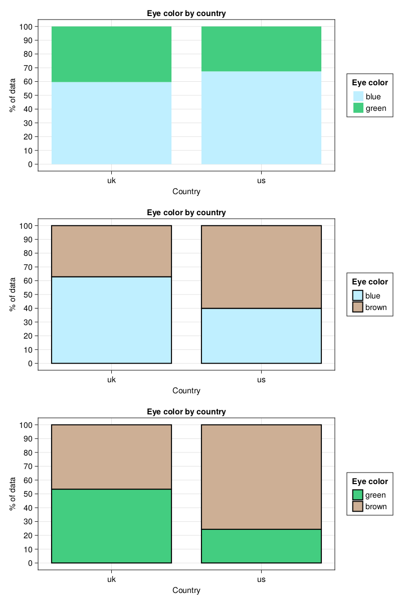
It looks quite OK + it allows us to quickly judge which eye colors distributions differ one from another. For a more complicated layout we should probably follow the guidelines contained in the Layout Tutorial.