5.7 Exercises - Comparisons of Continuous Data

Just like in the previous chapters here you will find some exercises that you may want to solve to get from this chapter as much as you can (best option). Alternatively, you may read the task descriptions and the solutions (and try to understand them).

5.7.1 Exercise 1

In Section 5.2 we said that when we draw a small random sample from a normal distribution of a given mean (\(\mu\)) and standard deviation (\(\sigma\)) then the distribution of the sample means will be pseudo-normal with the mean roughly equal to the population mean and the standard deviation roughly equal to sem (standard error of the mean).

Time to confirm that. Moreover, it’s time to practice our plotting skills (I think we neglected them so far).

In this task your population of interest is Dsts.Normal(80, 20). To make it more concrete let’s say this is the distribution of body weight for adult humans. To plot you may use CairoMakie or some other plotting library (read the tutorial(s)/docs first).

1. draw a random sample of size 10 from the population Dsts.Normal(80, 20). Calculate sem and sd for the sample,
2. draw 100’000 random samples of size 10 from the population Dsts.Normal(80, 200) and calculate the samples means (100’000 sample means)
3. draw the histogram of the sample means from point 2 using, e.g. Cmk.hist. Afterwards, you may set the y-axis limits from 0 to 4000, with Cmk.ylims!(0, 4000).
4. on the histogram mark the population mean (\(\mu = 80\)) with a vertical line using, e.g. Cmk.vlines
5. annotate the line from point 4 (e.g. type “population mean = 80”) using, e.g. Cmk.text
6. on the histogram mark the means standard deviation using, e.g. Cmk.bracket,
7. annotate the histogram (above the bracket from point 6) with the means standard deviation, using, e.g. Cmk.text,
8. annotate the histogram with the sample’s sem and sd (from point 1) and compare them with the means standard deviation from point 7.

And that’s it. This may look like a lot of work to do, but don’t freak out, do it one point at a time, look at the instructions (they are pretty precise on purpose).

Remember that each of those functions may have an equivalent that ends with ! (a function that modifies an already existing figure). It is for you to decide when to use which version of a plotting function.

5.7.2 Exercise 2

Do you remember how in Section 5.4 we calculated the L-statistic for ex2BwtsWater and ex2BwtsDrugY and found out its value was equal to LStatisticEx2 = 1.28? Then we calculated the famous F-statistic for the same two groups (ex2BwtsWater and ex2BwtsDrugY) and it was equal to getFStatistic(ex2BwtsWater, ex2BwtsDrugY) = 6.56. The probability of obtaining an F-value greater than this (by chance) if \(H_{0}\) is true (i.e. both groups come from the same distribution (Dsts.Normal(25, 3)) is equal to:

# the way we calculated it in the chapter (more or less)
Htests.OneWayANOVATest(ex2BwtsWater, ex2BwtsDrugY) |> Htests.pvalue

0.042836426298994756

Alternatively, we cold calculate it also with our friendly Distributions package (similarly to how we used it in, e.g. Section 4.6.2)

# the way we can calculate it with Distributions package
# 1 - Dfs for groups (number of groups - 1),
# 6 - Dfs for residuals (number of observations - number of groups)
1 - Dsts.cdf(Dsts.FDist(1, 6), getFStatistic(ex2BwtsWater, ex2BwtsDrugY))

0.042836426298994756

Hopefully, you remember that. OK, here is the task.

1. write a function getLStatistic(v1::Vector{<:Real}, v2::Vector{<:Real})::Float64 that calculates the L-Statistic for two given vectors

2. estimate the L-Distribution. To do that:

   2.1) run, let’s say 1’000’000 simulations under \(H_{0}\) that v1 and v2 come from the same population (Dsts.Normal(25, 3), draw 4 observations per vector). Calculate the L-Statistic each time (round it to 1 decimal place with round(getLStatistic(v1, v2), digits=1)

   2.2) use getCounts (Section 4.4), getProbs (Section 4.4) and getSortedKeysVals (Section 4.5) to obtain the probabilities for each value of the L-Statistic produced in point 2.1

   2.3) based on the data from point 2.2 calculate the probability of L-Statistic being greater than LStatisticEx2 = 1.28. Compare the probability with the probability obtained for the F-Statistic (presented in the code snippets above)

3. using, e.g. Cmk.lines (color="blue") and the data from point 2.2 plot the probability distribution for the L-Distribution

4. add vertical line, e.g with Cmk.vlines at L-Statistic = 1.28, annotate the line with Cmk.text

5. check what happens if both the samples from point 2.1 come from a different population (e.g. Dsts.Normal(100, 50)). Plot the new distribution on the old one (point 3) with, e.g. Cmk.scatter (marker=:circle, color="blue").

6. check what happens if the samples from point 2.1 come from the same distribution (Dsts.Normal(25, 3)) but are of different size (8 observations per vector). Plot the new distribution on the old one (point 3) with, e.g. Cmk.scatter (marker=:xcross, color="blue").

Optionally, if you want to make your plots more readable and if you like challenges you may:

7. add the F-Distribution to the plot, e.g. with Cmk.lines (color="red")
8. add legends to the plots

Again. This may look like a lot of work to do, but don’t freak out, do it one point at a time, look at the instructions (they are pretty precise on purpose). If you get stuck, take a sneak peak at the solution and continue on your own once you get back on the track.

5.7.3 Exercise 3

Let’s cool down after the last two demanding exercises.

In this task I want you to write the function getPValUnpairedTest(v1::Vector{<:Real}, v2::Vector{<:Real})::Float64. The function accepts two vectors, runs an unpaired test and returns the p-value.

The function should check the:

1. normality (Pg.normality), and
2. homogeneity of variance (Htests.FlingerTest)

assumptions.

If both the assumptions hold then run Htests.EqualVarianceTTest.

If only normality assumption holds then run Htests.UnequalVarianceTTest.

Otherwise run Htests.MannWhitneyUTest.

5.7.4 Exercise 4

Write a function with the following signature:

function getPValsUnpairedTests(
    df::Dfs.DataFrame
    )::Dict{Tuple{String,String},Float64}

The function accepts a data frame (like miceBwtABC we met in Section 5.5). Then it runs the appropriate comparisons (use getPValUnpairedTest that you developed in Section 5.7.3) and returns the p-values for comparisons in the form of a dictionary where the keys are the names of the compared groups (Tuple{String, String}), and the values are pvalues (e.g. Dict(("grX", "grY") => 0.3, ("grX", "grZ") => 0.022). The function should compare every group with every other group.

Once you are done with this task tweak your function slightly to have the following signature:

function getPValsUnpairedTests(
    df::Dfs.DataFrame,
    multCorr
    )::Dict{Tuple{String,String},Float64}

This function adjusts the obtained p-values using some sort of multiplicity correction (multCorr) from MultipleTesting package we discussed before (Section 5.6). I didn’t write the type signature for multCorr here because it might be frightening at first sight. Still, even without it the function should work just fine.

Test your function on miceBwtABC and compare the results with those we obtained in Section 5.5 and in Section 5.6.

5.7.5 Exercise 5

It appears that when a scientific paper presents a comparison between few groups of continuous variables it does so in a form of bar-plot or box-plot with some markers for statistically significant differences over the bars/boxes.

So here is your task. For data from miceBwtABC from Section 5.5 write a function that draws a plot similar to the one below (it doesn’t have to be the exact copy).

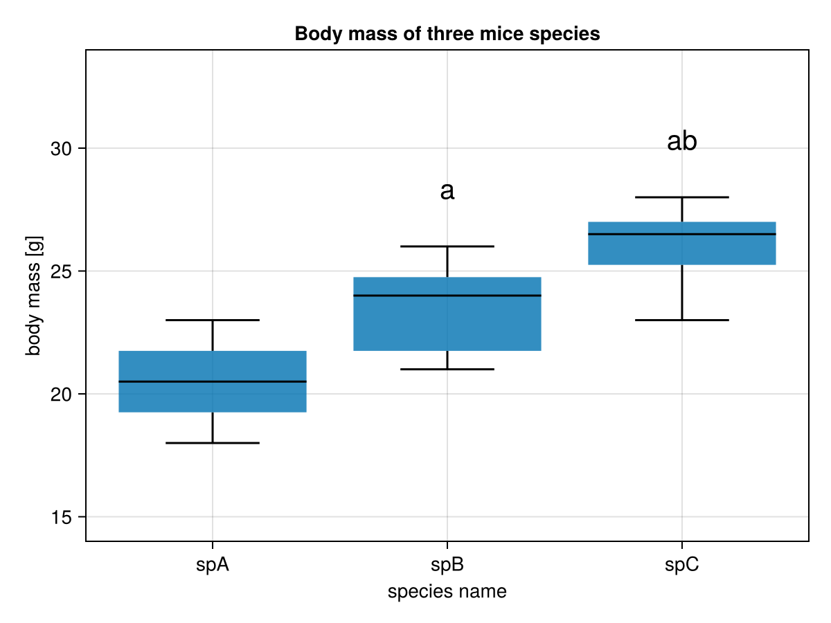
In the graph a middle horizontal line in a box is the median, a box depicts interquartile range (IQR), the whiskers length is equal to 1.5 * IQR (or the maximum and minimum if they are smaller than 1.5 * IQR).

For the task you may use:

• Cmk.boxplot - to draw the boxplot
• Cmk.xticks - to add group labels in x-ticks
• p-values provided by getPValsUnpairedTests(miceBwtABC, Mt.BenjaminiHochberg) from the last exercise to generate statistical significance markers.
• Cmk.text to place the markers in the correct positions on the plot.

The function should also work for different data frames of similar kind with different number of groups in the columns.